Assignment 5

Resources:

• Single-Target Tracking

---

Task 1: State dependent detection probability

We have

$$\begin{array}{rl}p(x|\delta )& =\frac{Pr(\delta |x)p(x)}{Pr(\delta )}\\ p(x|\delta )& =\frac{P_D(x)p(x)}{\int P_D(x)p(x)dx}\end{array}$$

From this we can see that $p(x|\delta )=p(x)$ only when $P_D(x)$ is a constant.

$$\begin{array}{rl}p(x|\delta )& =\frac{P_D\cdot p(x)}{P_D\int p(x)dx}\\ p(x|\delta )& =p(x)\end{array}$$

Since $\int p(x)dx=1$.

Otherwise, when $P_D(x)$ is non-constant we have $p(x|\delta )\ne p(x)$.

$$p(x|\delta )=\{\begin{array}{ll}p(x),& \text{For }{P}_D\text{ constant}\\ \ne p(x),& \text{otherwise}\end{array}$$

Task 2: The PDAF event probabilities

a)

We have a hit or miss type of probability over several samples, therefore a binomial distribution is logical.

$$\begin{array}{rl}Pr(\varphi )& =\text{Bin}(n=\varphi ,p=P_{FA})\\ Pr(\varphi )& =\left(\genfrac{}{}{0ex}{}{M_k}{\varphi }\right)P_{FA}^{\varphi }(1-P_{FA}{)}^{M_K-\varphi }\end{array}$$

b)

We can approximate this by

$$\lambda V_k=M_k{P}_{FA}$$

We want to prove

Starting from

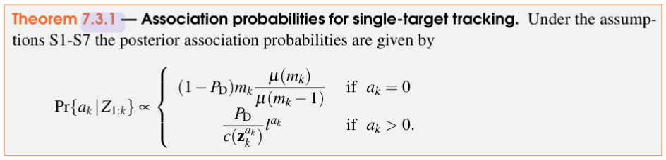
Starting with the case where $a_k=0$, and knowing that $\mu (\varphi =m_k,\Lambda =\lambda V_k)=\frac{e^{-\lambda V_k}(\lambda V_k{)}^{m_k}}{m_k!}$, we get:

$$\begin{array}{r}Pr(a_k=0|Z_{1:k})=(1-P_D)m_k\frac{\frac{e^{-\lambda V_k}(\lambda V_k{)}^{m_k}}{m_k!}}{\frac{e^{-\lambda V_k}(\lambda V_k{)}^{m_k-1}}{(m_k-1)!}}=(1-P_D)\lambda V_k\end{array}$$

While the case where $a_k>0$, and we know that

• $c(z_k)=\frac{1}{V_k}$
• $l^{a_k}=\mathcal{N}(z_k^{a_k};{\hat{z}}_{k:k-1},S_k)$, due to it being Gaussian-linear

we get:

$$\begin{array}{rl}Pr(a_k>0|Z_{1:k})& =\frac{P_D}{\frac{1}{V_k}}\mathcal{N}(z_k^{a_k};{\hat{z}}_{k:k-1},S_k)\\ Pr(a_k>0|Z_{1:k})& =V_k{P}_D\mathcal{N}(z_k^{a_k};{\hat{z}}_{k:k-1},S_k)\end{array}$$

Since we’re only looking at the proportionally sign, we can remove $V_k$ as it is a factor independent of $a_k$. We therefore get

$$Pr(a_k|Z_{1:k})\propto \{\begin{array}{ll}(1-P_D)\lambda ,& a_k=0\\ P_D\mathcal{N}(z_k^{a_k};{\hat{z}}_{k:k-1},S_k),& a_k>0\end{array}$$

c)

Same as the last task, but we swap from using the Poisson distribution to the binomial distribution found in a). Skipping some messy algebra, we get

$$Pr(a_k|Z_{1:k})\propto \{\begin{array}{ll}(1-P_D)\frac{M_k{P}_{FA}\left(1-\frac{m_k-1}{M_k}\right)}{V_k(1-P_{FA})},& a_k=0\\ P_D\mathcal{N}(z_k^{a_k};{\hat{z}}_{k:k-1},S_k),& a_k>0\end{array}$$

Q.E.D

d)

We know from b) that $\lambda V_k=M_k{P}_{FA}$, and from the hint we can rewrite the distribution in $c)$ to become

$$Pr(a_k|Z_{1:k})\propto \{\begin{array}{ll}(1-P_D)\frac{\lambda V_k\left(1-0\right)}{V_k(1-0)}=(1-P_D)\lambda ,& a_k=0\\ P_D\mathcal{N}(z_k^{a_k};{\hat{z}}_{k:k-1},S_k),& a_k>0\end{array}$$

Which is the exact same distribution that we found in b). This means that our approximation is good when $M_k$ is large and $P_{FA}$ is small.

Task 3: IPDA vs PDAF

Resources:

• PDAF
• IPDA

a)

[!Task description] Briefly discuss why the posterior becomes a mixture in single target tracking. In particular, what is the interpretation of a component and its weight. What are the main complicating factors of this mixture?

In single target tracking we have several measurements, and we do not know which one is the correct one. We therefore have to consider a mixture of these (Gaussian) measurements where each measurement is weighted by the probability of it being the correct measurement.

b)

[!Task description] What problem does the IPDA try to solve that the PDA does not? Are there any problems that the PDA solves which the IPDA does not solve?

The PDAF assumes the target is always present. Its main focus is figuring out which measurements actually come from the target and which ones are just noise or false alarms. This makes it highly accurate and effective when the target is definitely there.

The IPDA extends this, and considers that the target might disappear over time, keeping track of the probability that the target actually exists. This means IPDA can “kill” them when it’s no longer there, making it useful for handling more complex tracking scenarios.

Therefore, the PDAF does not solve any problems that the IPDA doesn’t already solve.

c)

A complicating factor of using IPDA instead of the PDAF is another tuning variable, $P_S$ (the probability that the target survives), and the extra compute needed to update this variable.

Task 4: Implement a parametric PDAF

a)

The validation gate is given by

$$\mathcal{G}=\{z\text{ such that }(z-{\hat{z}}_{k|k-1}{)}^T(S_k^{-1})(z-{\hat{z}}_{k|k-1})<g^2\}$$

This is done by updating the variable condition to be

from scipy.spatial.distance import mahalanobis
 
condition = mahalanobis(z, z_est_pred.mean, np.linalg.inv(z_est_pred.cov)) ** 2 < self.gate

b)

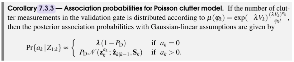
The formula we want to implement is given by

$$Pr\{a_k|Z_{1:k}\}\propto \{\begin{array}{ll}\lambda (1-P_D)& \text{if }{a}_k=0\\ P_D\mathcal{N}(z_k^{a_k};{\hat{z}}_{k|k-1},{\mathcal{S}}_k)& \text{if }{a}_{k>0}\end{array}$$

This is done by updating the variable assoc_probs

def get_assoc_probs(self, z_est_pred: MultiVarGauss[MeasPos],
                        zs: Sequence[MeasPos]) -> np.ndarray:
        """Compute the association probabilities.
        P{a_k|Z_{1:k}} = assoc_probs[a_k]    (corollary 7.3.3)
 
        Hint: use some_gauss.pdf(something), rememeber to normalize"""
        lamb = self.sensor_model.clutter_density
        P_D = self.sensor_model.prob_detect
 
        assoc_probs = np.empty(len(zs) + 1)
 
        assoc_probs[0] = lamb * (1 - P_D)
        for i, z in enumerate(zs):
            assoc_probs[i+1] = P_D * z_est_pred.pdf(z)
        
        assoc_probs /= np.sum(assoc_probs)
 
        return assoc_probs

c)

We want to update ${\hat{x}}_k^{a_k}$ based on the update rule

$${\hat{x}}_k^{a_k}=\{\begin{array}{ll}{\hat{x}}_{k|k-1}& \text{if }{a}_k=0\\ {\hat{x}}_{k|k-1}+W_k{\nu }_k^{a_k}& \text{if }{a}_k>0\end{array}$$

This is done by updating the variable x_ests

def get_estimates(self,
                      x_est_pred: MultiVarGauss[StateCV],
                      z_est_pred: MultiVarGauss[MeasPos],
                      zs_gated: Sequence[MeasPos]
                      ) -> Sequence[MultiVarGauss[StateCV]]:
        """Get the estimates corresponding to each association hypothesis.
 
        Compared to the book that is:
        hat{x}_k^{a_k} = x_ests[a_k].mean   (7.20)
        P_k^{a_k} = x_ests[a_k].cov         (7.21)
 
        Hint: Use self.ekf"""
        x_ests = []
        gauss_ak0 = x_est_pred
        x_ests.append(gauss_ak0)
        for z in zs_gated:
            x_est_upd = self.ekf.update(x_est_pred, z_est_pred, z)
            x_ests.append(x_est_upd)
 
        return x_ests

d)

Here we want to combine the previous tasks as well as some equations from the book.

def step(self,
             x_est_prev: MultiVarGauss[StateCV],
             zs: Sequence[MeasPos],
             dt: float) -> tuple[MultiVarGauss[StateCV],
                                 MultiVarGauss[StateCV],
                                 MultiVarGauss[MeasPos],
                                 set[int]]:
        """Perform one step of the PDAF."""
 
        x_est_pred, z_est_pred = self.ekf.pred(x_est_prev, dt)   # Hint: (7.16) and (7.17)
        gated_indices, zs_gated = self.gate_zs(z_est_pred, zs) # Hint: (7.3.5)
        assoc_probs = self.get_assoc_probs(z_est_pred, zs_gated)  # Hint: (7.3.3)
        x_ests = self.get_estimates(x_est_pred, z_est_pred, zs_gated)  # Hint: (7.20) and (7.21)
 
        weighted_mean = 0
        weighted_covariance = 0
 
        for prob, estimate in zip(assoc_probs, x_ests):
            weighted_mean += prob * estimate.mean
 
        for prob, estimate in zip(assoc_probs, x_ests):
            mean_deviation = estimate.mean - weighted_mean
            weighted_covariance += prob * (estimate.cov + np.outer(mean_deviation, mean_deviation))
 
        x_est_upd = MultiVarGauss(weighted_mean, weighted_covariance)
 
 
        return x_est_upd, x_est_pred, z_est_pred, gated_indices

Task 5: Tune your parametric PDAF

a)

The approach of increasing the gate probability when the estimated acceleration noise is high is an approach that works, however the state estimations are less accurate this way.

b)

Makes the tracking worse, and at some point it will diverge.

c)

If one does not have access to any ground truth states, it is impossible to detect this behaviour.

(However, it could be detected if the object were placed in a known position over time (and not moving), and looking for divergence. This is not possible since we don’t have GT).

d)

Using IMM and better tuning.