Exercise 5 - Open-Loop Optimal Control and MPC

Problem 1 (60%) Open-Loop Optimal Control

We have the model

$$\begin{array}{rl}{x}_{t+1}& =\underset{A}{\underbrace{\left[\begin{array}{ccc}0& 0& 0\\ 0& 0& 1\\ 0.1& -0.79& 1.78\end{array}\right]}}{x}_t+\underset{B}{\underbrace{\left[\begin{array}{c}1\\ 0\\ 0.1\end{array}\right]}}{u}_t\\ y_t& =\underset{C}{\underbrace{\left[\begin{array}{ccc}0& 0& 1\end{array}\right]}}{x}_t\end{array}$$

The process has been at $x_t=0$, $u_t=0$, but at $t=-1$ a disturbance moves it to $x_0=[0,0,1{]}^T$. We wish to solve a Finite Horizon LQR ($N<\infty$) with the cost (or objective) function

$$f(y_1,\dots ,y_N,u_0,\dots ,u_{N-1})=\sum _{t=0}^{N-1}\{y_{t+1}^2+r{u}_t^2\},r>0$$

Where $r=1$ (for the time being), and $N=30$

a) Eigenvectors and Eigenvalues

For a discrete, causal system to be stable, we need to have eigenvalues with absolute value smaller than $1$.

Using WolframAlpha we get that the eigenvalues of $A$ are

$$\begin{array}{rl}{\lambda }_1& \approx 0.94\\ {\lambda }_2& \approx 0.84\\ {\lambda }_3& =0\end{array}$$

The system is therefore stable.

b)

$x_t$ is a $3\times 1$ vector, while $u_t$ is a $1\times 1$ matrix for the dimensions to match

If we set $z=[x_1^T,\dots ,x_N^T,u_0^T,\dots ,u_{N-1}^T{]}^T$, we can rewrite the cost function as

$$f(z)=\frac{1}{2}\sum _{t=0}^{N-1}\{x_{t+1}^{T}Q{x}_{t+1}+u_t^{T}R{u}_t\}$$

We now need to find $Q$ and $R$.

We know that

$$y_t=C{x}_t=\left[\begin{array}{ccc}0& 0& 1\end{array}\right]x_t$$

Which means that we can write $Q$ as

$$Q=\left[\begin{array}{ccc}0& 0& 0\\ 0& 0& 0\\ 0& 0& 2\end{array}\right]$$

Note that the reason that we have $2$ in the bottom left is due to the general form of LQR has a $\frac{1}{2}$ in front.

Similarly we can write $R$ as

$$R=2r$$

c)

When we have $f(z)$ as a objective function, we need to look at $Q$ and $R$ to determine if the minimization problem is convex. Since $Q$ is a Positive-Semidefinite Matrix, and $R$ is a Positive-Definite Matrix, the QP is convex.

If $Q$ also was a Positive-Definite Matrix, then the problem would be strictly convex.

In other words, convexity depends solely on $Q$ and $R$.

d) Equality-Constrained Quadratic Programs

We will now cast the optimal control problem as a equality-constrained QP.

$$\underset{z}{\min }f(z)=\frac{1}{2}{z}^{T}Gzs.t.A_{eq}z=b_{eq}$$

---

Each row in the constraint $A_{eq}z=b_{eq}$ represents the state equation for a time instant. That is the reason for the structure given.

With the same reasoning we can define $G$ as

$$G=\left[\begin{array}{cccccc}Q& 0& \dots & \dots & \dots & 0\\ 0& \ddots & \ddots & & & ⋮\\ ⋮& \ddots & Q& \ddots & & ⋮\\ ⋮& & \ddots & R& \ddots & ⋮\\ ⋮& & & \ddots & \ddots & 0\\ 0& \dots & \dots & \dots & 0& R\end{array}\right]$$

We know that the KKT Matrix for Equality-Constrained QPs is given as

Link to original

Where $A=A_{eq}$, $b=b_{eq}$, and $c=0$.

We can solve the open-loop optimal control problem with the following Matlab script.

% Define the system dynamics matrices
A = [0,    0,    0;
     0,    0,    1;
     0.1, -0.79, 1.78];
B = [1; 0; 0.1];
C = [0, 0, 1];
 
% Initial state
x0 = [0; 0; 1];
 
% Set the control horizon
N = 30;
 
% Determine the number of states and controls
nx = size(A, 2); 
nu = size(B, 2); 
 
% Define the cost matrices
Qt = 2 * diag([0, 0, 1]);
Rt = 2;
I_N = sparse(eye(N));
Q = sparse(kron(I_N, Qt));
R = sparse(kron(I_N, Rt));
G = blkdiag(Q, R);
 
% Construct the equality constraint matrices
Aeq_c1 = sparse(eye(N * nx));                          % Identity matrix for x
Aeq_c2 = sparse(kron(diag(ones(N-1, 1), -1), -A));     % Shifted dynamics matrix
Aeq_c3 = sparse(kron(I_N, -B));                        % Control dynamics
Aeq = [Aeq_c1 + Aeq_c2, Aeq_c3];
beq = sparse([A * x0; zeros((N - 1) * nx, 1)]);
 
% Initialize zero matrices for KKT system formulation
zero_m = sparse(zeros(N * nx));
zero_v = sparse(zeros(N * (nx + nu), 1));
 
% Assemble the KKT system
KKT_mat = [G,    -Aeq';
           Aeq,  zero_m];
KKT_vec = [zero_v; beq];
 
% Solve the KKT system for optimal trajectory
KKT_sol = KKT_mat \ KKT_vec;
 
% Extract solution for plotting
z = KKT_sol(1:N * (nx + nu)); % Solution vector
y = [x0(3); z(nx:nx:N * nx)]; % Extract y_t from solution
u = z(N * nx + 1:end);        % Extract control inputs
 
% Correct the time vector to include the initial step for plotting
t = 0:N; % Now t ranges from 0 to N, making it have N+1 elements
 
% Plot adjustments to match the corrected time vector
figure(1);
subplot(2, 1, 1);
plot(t, y, '-ko'); % Plot y_t over the control horizon, ensuring t and y have the same length
grid on;
ylabel('y_t');
title('Optimal Trajectory');
 
% Assuming u is plotted correctly against t-1 in the original code
subplot(2, 1, 2);
plot(t(1:end-1), u, '-ko'); % Plot control inputs over the control horizon, excluding the last element of t to match u's length
grid on;
xlabel('Time step, t');
ylabel('Control input, u_t');
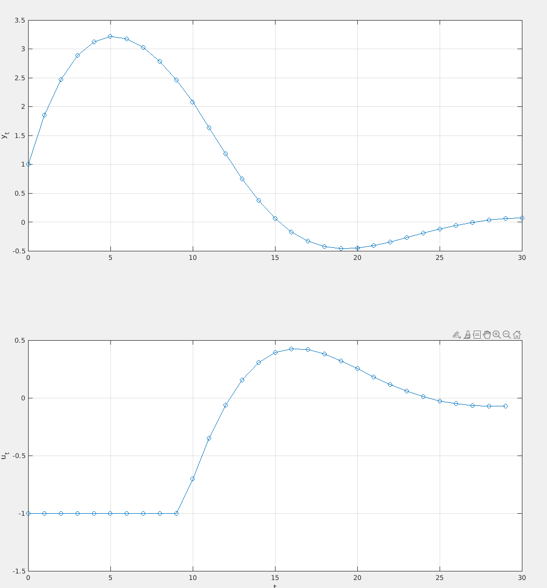
title('Control Inputs');

Yielding the following plot

---

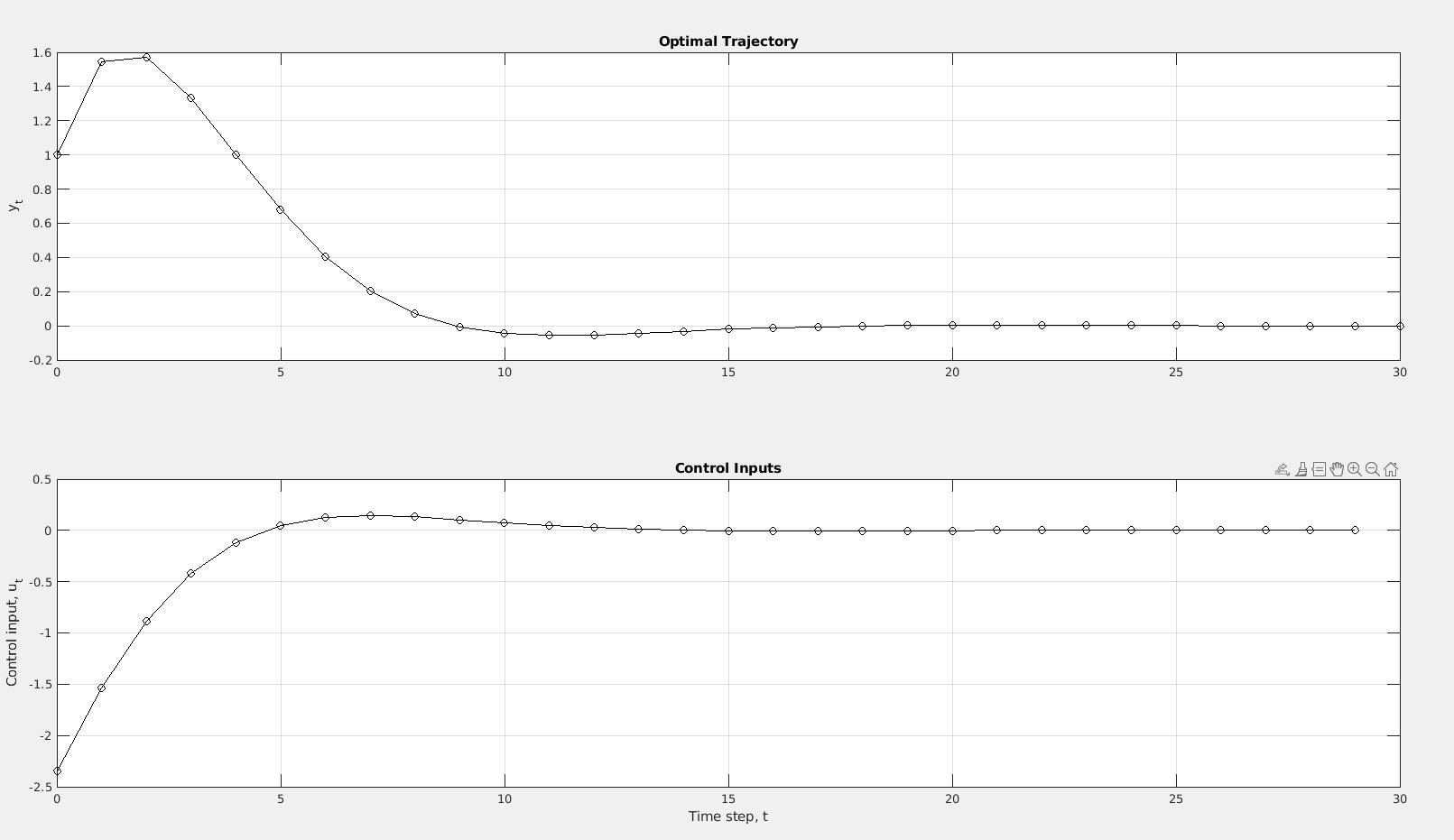
Why do we call this open-loop control? We call this for an open-loop control sequence due to not having new measurements after the system has started. Open-loop = no feedback.

What are the advantages of including feedback…? Including feedback into the system can make up for not having a perfect model (which is impossible irl) or other disturbances.

…and how can this be accomplished? We could include feedback by calculating the optimal path again after each new measurement. Although this would be compute heavy, it would also be way more accurate.

e)

While d) focused on solving the problem with the KKT system, we will in this sub task solve the QP directly using the quadprog function.

Modifying the script gives us the following figures with one iteration of quadprog

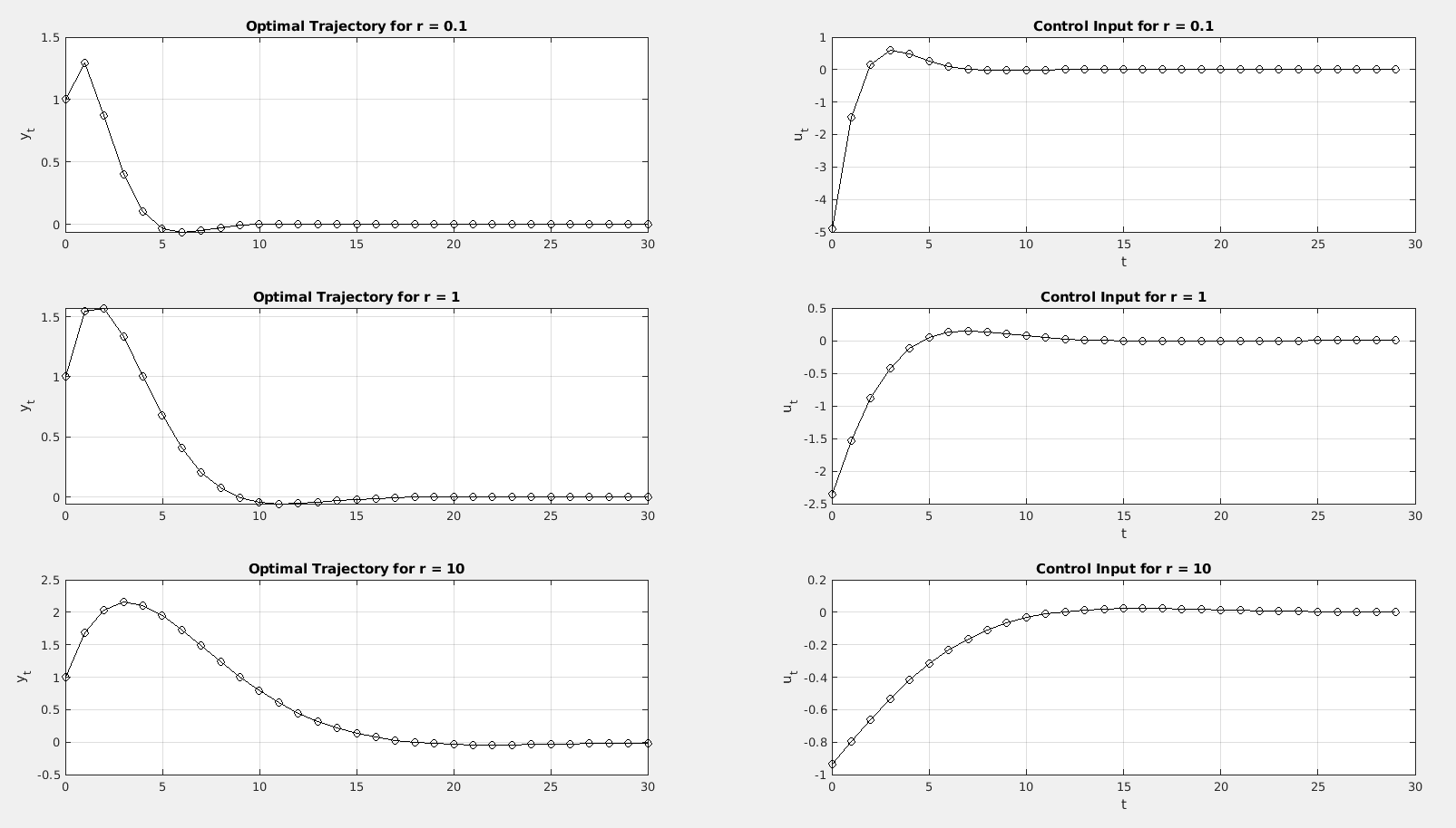
We see that for lower values of $r$, we have more aggressive control due to decreasing the cost of using energy.

f)

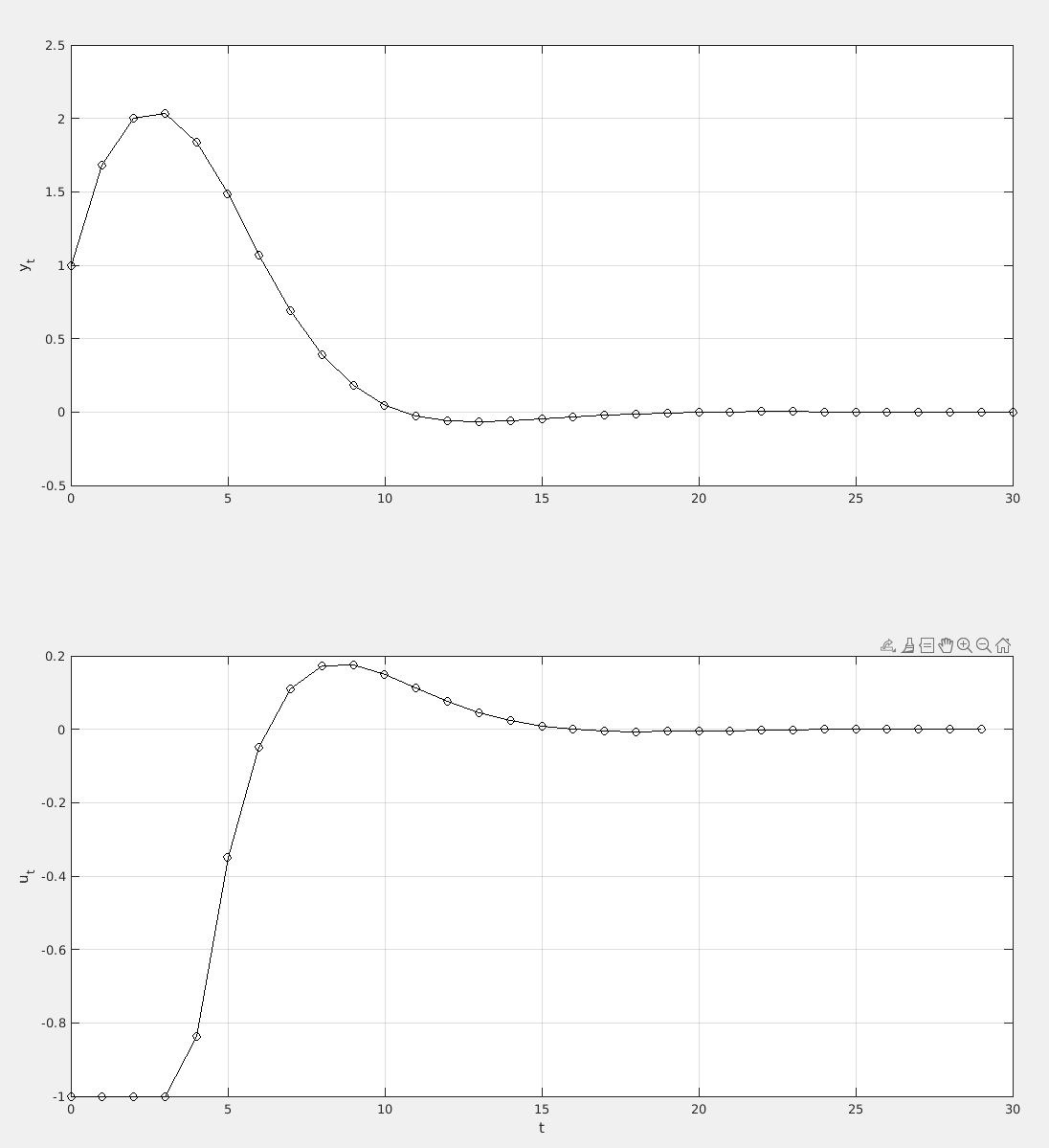
We adjust $z$ such that we have no constraints on $x$ ($-\infty <x<\infty$), and the following constraint for $u$, $-1\le u_t\le 1,t\in [0,N-1]$.

This is done the following way.

% Inequality constraints
x_lb = -Inf(N*nx,1);    % Lower bound on x
x_ub =  Inf(N*nx,1);    % Upper bound on x
u_lb = -ones(N*nu,1);   % Lower bound on u
u_ub =  ones(N*nu,1);   % Upper bound on u
lb = [x_lb; u_lb];      % Lower bound on z
ub = [x_ub; u_ub];      % Upper bound on z

And then lb and ub is passed to quadprog.

Which yields

Problem 2 (40%) Model Predictive Control (MPC)

a)

A way to control a process while satisfying the set of constraint. A model of the process is used to compute the control signals (inputs) that optimize predicted future process behavior.

Link to original

More technically, we calculate a finite horizon open-loop optimal control problem at each time instant, which is based on the current measurement.

We set $x_0=x(t)$, which is our feedback. This is the reason our process looks like it does in the graph.

Link to original

b)

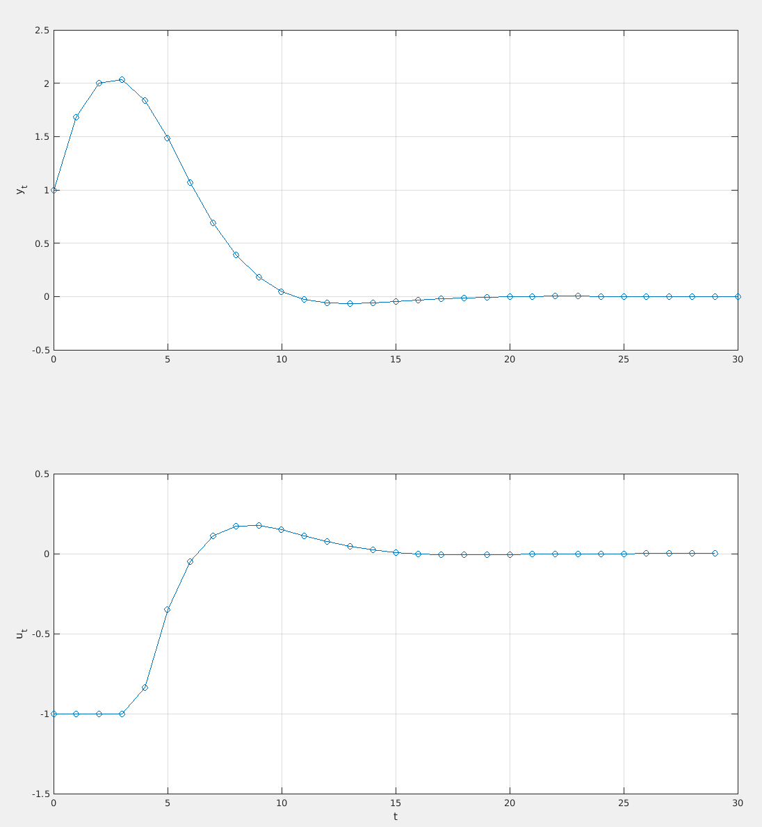
The main difference is that we now iterate over every discrete time step, and calculate the optimization problem with $z_0=z(t)$.

Since we assumed a perfect model, the result is near identical

c)

Now, using the real plant instead, we see that the MPC still manages to reach the setpoint of $0$, but not as good as when we had a perfect model. This is done in the same way as b), but when moving a time step ahead, we extract the current state from the real plant, and not the model.