LinSys Assignment 3

Problem 1

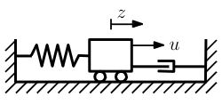
Given the following equation for the system

$$\ddot{y}(t)+\dot{y}(t)+2y(t)=2u(t)$$

a) We can rewrite the system on State Space Representation form, where

$$x(t)=\left[\begin{array}{c}{x}_1(t)\\ x_2(t)\end{array}\right]=\left[\begin{array}{c}y(t)\\ \dot{y}(t)\end{array}\right]$$

Gives us

\dot{x_{1}} &= x_{2} \\ \dot{x_{2}} &= 2u-2x_{1}-x_{2} \end{align}

Which on state space form is

\dot{x} &= \begin{bmatrix} 0 & 1 \\ -2 & -1 \end{bmatrix}x+\begin{bmatrix} 0 \\ 2 \end{bmatrix}u \\ y &= \begin{bmatrix} 1 & 0 \end{bmatrix}x \end{align}

Where

$$A=\left[\begin{array}{cc}0& 1\\ -2& -1\end{array}\right],B=\left[\begin{array}{c}0\\ 2\end{array}\right],C=\left[\begin{array}{cc}1& 0\end{array}\right]$$

b) We can write the controller as

$$u(t)=u_{eq}+\tilde{u}(t)$$

Where $u_{eq}$ is the feedforward part of the controller, and $\tilde{u}(t)$ is the feedback of the controller. We now want to find the equilibrium point of the system

$$\begin{array}{rl}(1)x_{eq}& =-A^{-1}B{u}_{eq}=\frac{1}{2}\left[\begin{array}{cc}-1& -1\\ 2& 0\end{array}\right]\left[\begin{array}{c}0\\ 2\end{array}\right]u_{eq}=\left[\begin{array}{c}1\\ 0\end{array}\right]u_{eq}\\ (2)r& =C{x}_{eq}=C\left[\begin{array}{c}1\\ 0\end{array}\right]u_{eq}=u_{eq}\end{array}$$

Giving us that $u_{eq}=Gr$, and $x_{eq}=Fr$ where

$$F=\left[\begin{array}{c}1\\ 0\end{array}\right],G=1$$

$Q.E.D$

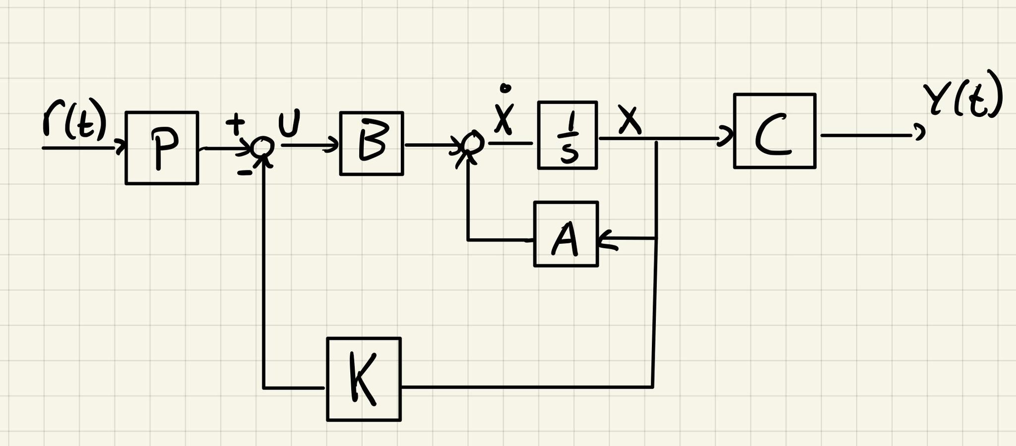
c) Given the state error on State Space Representation form

$$\begin{array}{r}\dot{\tilde{x}}=A\tilde{x}+B\tilde{u}\\ \tilde{y}=C\tilde{x}\end{array}$$

And we have the following LQR cost function (State Feedback, and Optimal Control)

$$J={\int }_0^{\infty }[{\tilde{x}}^{T}Q\tilde{x}+R{\tilde{u}}^2]dt$$

and the control input

$$\tilde{u}=-K\tilde{x}$$

Where $K=R^{-1}{B}^{T}P$, and the Positive-Definite Matrix P is the solution of the Algebraic Ricatti Equation.

Algebraic Ricatti Equation

A type of nonlinear equation that arises in the context of infinite-horizon optimal control problems in continuous or discrete time.

---

Continuous time algebraic Riccatti equation

$$A^{T}P+PA-PB{R}^{-1}{B}^{T}P+Q=0$$

Where $P$ is an unknown $n\times n$ Positive-Definite Matrix

Positive-Definite Matrix

A symmetric matrix with all positive eigenvalues. NOTE: All symmetric matrices have only real eigenvalues

For a matrix, $M$, to be positive-semidefinite the following has to hold

Criterion

$x^{T}Mx>0,\forall x\in {\mathbb{R}}^n\backslash \{0\}$ Given that $M$ is a $n\times n$ symmetric real matrix

---

Can be written generally as

$$M=\left[\begin{array}{cc}{m}_1& m_2\\ m_2& m_3\end{array}\right]$$Link to original

Link to original

Given

$$R=4,Q=\left[\begin{array}{cc}5& 0\\ 0& 1\end{array}\right]$$

We get (Using WolframAlpha)

\begin{bmatrix} 0 & -2 \\ 1 & -1 \end{bmatrix} \begin{bmatrix} p_{1} & p_{2} \\ p_{2} & p_{3} \end{bmatrix} +\begin{bmatrix} p_{1} & p_{2} \\ p_{2} & p_{3} \end{bmatrix} \begin{bmatrix} 0 & 1 \\ -2 & -1 \end{bmatrix} -\begin{bmatrix} p_{1} & p_{2} \\ p_{2} & p_{3} \end{bmatrix} \begin{bmatrix} 0 \\ 2 \end{bmatrix} 4^{-1} \begin{bmatrix} 0 & 2 \end{bmatrix} \begin{bmatrix} p_{1} & p_{2} \\ p_{2} & p_{3} \end{bmatrix} +\begin{bmatrix} 5 & 0 \\ 0 & 1 \end{bmatrix} &=0\\ \dots \\ \begin{bmatrix} -4p_{2}-p_{2}²+5 & p_{1}-p_{2}-2p_{3}-p_{2}p_{3} \\ p_{1}-p_{2}-2p_{3}-p_{2}p_{3} & 2p_{2}-2p_{3}-p_{3}²+1 \end{bmatrix} &=0 \end{align}

We now solve the 3 unique equations, and obtain following values for $p_1,p_2,p_3$

$$\begin{array}{rl}& \\ p_1& =p_2+2p_3+p_2{p}_3\\ p_2& =-2\pm 3\\ p_3& =-1\pm \sqrt{2(p_2+1)}\end{array}$$

We need $P$ to be a Positive-Definite Matrix, aka positive eigenvalues

$$\det (P)=p_1{p}_3-p_2^2>0$$

Which obtain the following four unique solutions For $p_2=1$

$$P_1=\left[\begin{array}{cc}4& 1\\ 1& 1\end{array}\right]P_2=\left[\begin{array}{cc}-8& 1\\ 1& -3\end{array}\right]$$

For $p_2=-5$

$$P_3=\left[\begin{array}{cc}-2-6\sqrt{2}j& -5\\ -5& -1+2\sqrt{2}j\end{array}\right]P_4=\left[\begin{array}{cc}-2+6\sqrt{2}j& -5\\ -5& -1-2\sqrt{2}j\end{array}\right]$$

Where $\det (P_2,P_3,P_4)\le 0$, and $\det (P_1)>0$. Therefore we must have

$$P=P_1=\left[\begin{array}{cc}4& 1\\ 1& 1\end{array}\right]$$

Which gives us

$$K=R^{-1}{B}^{T}P=4^{-1}\left[\begin{array}{cc}0& 2\end{array}\right]\left[\begin{array}{cc}4& 1\\ 1& 1\end{array}\right]=\left[\begin{array}{cc}\frac{1}{2}& \frac{1}{2}\end{array}\right]$$

$Q.E.D$

e) The controller is previously given by:

$$u(t)=u_{eq}+\tilde{u}(t)$$

Which we can rewrite to:

$$\begin{array}{rl}u& =Gr-K\tilde{x}(t)\\ u& =Gr-K(x-x_{eq})\\ u& =Gr-K(x-Fr)\\ u(t)& =-Kx(t)+pr\end{array}$$

Where $p=G+KF$

$$p=1+\left[\begin{array}{cc}\frac{1}{2}& \frac{1}{2}\end{array}\right]\left[\begin{array}{c}1\\ 0\end{array}\right]=\frac{3}{2}$$

f)

g) We need to prioritize the state ${\tilde{x}}_1=y$ (and therefore implicitly penalizing the rest). We can do this by increasing the first element in $Q$, so that the ratio between the first and last element is larger. This will make the controller worse at regulating the speed (${\tilde{x}}_2$), and since $R$ is down prioritized, the system will allow more energy to be spent, leading to higher values of $u$.

Problem 2

a) & b)

Transclude of Realizations#^93dba4

We have the transfer functions

$$\hat{G}(s)=\left[\begin{array}{cc}\frac{s^2+4s+2}{s^2+2s}& \frac{3}{s+2}\\ 0& \frac{2s^2}{s^2-4}\end{array}\right]$$

We can see this as the degree of the denominator is larger than or equal to the degree of the numerator (It is proper). The degree of the transfer function is also finite (it is rational). The system is realizable

c) We find $D$ by looking at the limit

$$D=\underset{s\to \infty }{\lim }\hat{G}(s)=\left[\begin{array}{cc}{\lim }_{s\to \infty }\frac{s^2+4s+2}{s^2+2s}& {\lim }_{s\to \infty }\frac{3}{s+2}\\ 0& {\lim }_{s\to \infty }\frac{2s^2}{s^2-4}\end{array}\right]=\left[\begin{array}{cc}1& 0\\ 0& 2\end{array}\right]$$

And then we can find ${\hat{G}}_{sp}(s)$ by solving

&\hat{G}_{sp}(s) = \hat{G}(s) - D \\ &= \begin{bmatrix} \frac{s²+4s+2}{s²+2s} - 1 & \frac{3}{s+2} \\ 0 & \frac{2s²}{s²-4} - 2 \end{bmatrix} \\ &=\dots \\ & \hat{G}_{sp}(s)=\begin{bmatrix} \frac{2s+2}{s²+2s} & \frac{3}{s+2} \\ 0 & \frac{s}{s²-4} \end{bmatrix} \end{align}

d) For simplicity, we rewrite the elements of ${\hat{G}}_{sp}$ as

$${\hat{G}}_{sp}=\left[\begin{array}{cc}a& b\\ 0& c\end{array}\right]$$

Where

$$\begin{array}{rl}a& =\frac{n_a}{d_a}=\frac{2s+2}{s^2+2s}\\ b& =\frac{n_b}{d_b}=\frac{3}{s+2}\\ c& =\frac{n_c}{d_c}=\frac{8}{s^2-4}\end{array}$$

The least common demoninator is $s(s+2)(s-2)$, and from the expressions $d(s)$ we get

$$d(s)=s^3+{\alpha }_1{s}^2+{\alpha }_{2}s+{\alpha }_3=s^3-4s$$

Meaning that ${\alpha }_1={\alpha }_3=0$ and ${\alpha }_2=4$

We now find our new expressions of ${\hat{G}}_{sp}$

$$\begin{array}{rl}{\hat{G}}_{sp}& =\left[\begin{array}{cc}\frac{2s+2}{s(s+2)}\cdot \frac{s-2}{s-2}& \frac{3}{s+2}\cdot \frac{s(s-2)}{(s(s-2))}\\ 0& \frac{s}{(s-2)(s+2)}\cdot \frac{s}{s}\end{array}\right]\\ {\hat{G}}_{sp}& =\frac{1}{s(s+2)(s-2)}\left[\begin{array}{cc}2s^2-2s-4& 3s^2-6s\\ 0& 8s\end{array}\right]\\ {\hat{G}}_{sp}& =\frac{1}{d(s)}(\left[\begin{array}{cc}2& 3\\ 0& 0\end{array}\right]s^2+\left[\begin{array}{cc}-2& -6\\ 0& 8\end{array}\right]s+\left[\begin{array}{cc}-4& 0\\ 0& 0\end{array}\right])\\ {\hat{G}}_{sp}& =\frac{1}{d(s)}(N_1{s}^2+N_{2}s+N_3)\end{array}$$

e) Using the values we found for the different alphas, $N$ matrices and $D$ gives us

$$\begin{array}{r}\dot{x}(t)=\left[\begin{array}{cccccc}0& 0& 4& 0& 0& 0\\ 0& 0& 0& 4& 0& 0\\ 1& 0& 0& 0& 0& 0\\ 0& 1& 0& 0& 0& 0\\ 0& 0& 1& 0& 0& 0\\ 0& 0& 0& 1& 0& 0\end{array}\right]x(t)+\left[\begin{array}{cc}1& 0\\ 0& 1\\ 0& 0\\ 0& 0\\ 0& 0\\ 0& 0\end{array}\right]u(t)\\ y(t)=\left[\begin{array}{cccccc}2& 3& -2& -6& -4& 0\\ 0& 0& 0& 8& 0& 0\end{array}\right]x(t)+\left[\begin{array}{cc}1& 0\\ 0& 2\end{array}\right]u(t)\end{array}$$

Where $I={\mathbb{I}}_2$

Problem 3

Given a system on State Space Representation form

Link to original

Where

$$A=\left[\begin{array}{cc}-4& 0\\ 3& -1\end{array}\right],B=\left[\begin{array}{c}2\\ 0\end{array}\right],C=\left[\begin{array}{cc}0& 1\end{array}\right],D=-2$$

a) The observability matrix is given by

Transclude of Observability#^9093bb

$$\mathcal{O}=\left[\begin{array}{c}C\\ CA\end{array}\right]=\left[\begin{array}{cc}0& 1\\ 3& -1\end{array}\right]$$

Since the observability matrix has full rank ($n=2$), the system is observable.

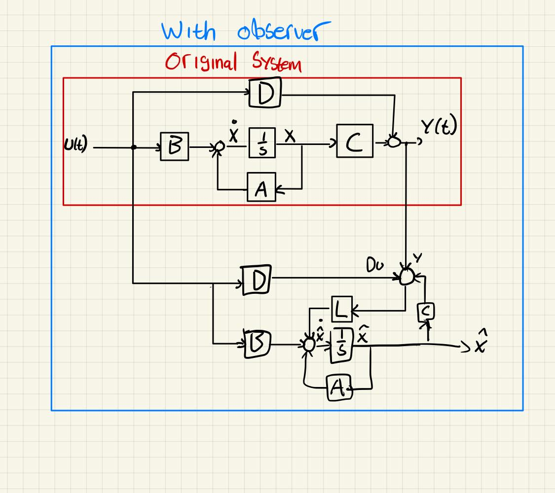
b) We have the following state estimator for the system

$$\dot{\hat{x}}=A\hat{x}+Bu+L(y-C\hat{x}-Du)$$

And since $e=x-\hat{x}$ and $\dot{e}=\dot{x}-\dot{\hat{x}}$

$$\begin{array}{rl}\dot{e}& =Ax-A\hat{x}+Bu-Bu+L(y-C\hat{x}-Du)\\ \dot{e}& =A(x-\hat{x})-L(Cx+Du-C\hat{x}-Du)\\ \dot{e}& =Ae-LCe\\ \dot{e}(t)& =(A-LC)e(t)\end{array}$$

$Q.E.D$

c) We place the poles in such a way that $\det (A-LC)=0$ yields ${\lambda }_1=-8$ and ${\lambda }_2=-10$. We set $L=[l_1,l_2{]}^T$ to simplify calculations

$$\det (A-LC)=\left|\begin{array}{cc}-4-\lambda & -l_1\\ 3& -1-l_2-\lambda \end{array}\right|={\lambda }^2+(5+l_2)\lambda +(4+3l_1+4l_2)$$

To get the correct eigenvalues, we want $(\lambda +8)(\lambda +10)={\lambda }^2+18\lambda +80$ We therefore get the following equations

$$\{\begin{array}{l}5+l_2=18\\ 4+3l_1+4l_2=80\end{array}$$

Which gives us

$$\begin{array}{r}{l}_2=13\\ l_1=8\end{array}$$

$L=[8,13{]}^T$ $Q.E.D$

d)

Problem 4

Given the following system

Link to original

Where $u(t)=-K\hat{x}(t)$, and the state estimator

$$\dot{\hat{x}}=A\hat{x}+Bu+L(y-C\hat{x}-Du)$$

a) The second row of the matrix corresponds to the expression we got in 3b). We will now find an expression for $\dot{x}$ in terms of the matrices $A,B,K$ and the states $x(t),e(t)$

$$\dot{x}=Ax-BK\hat{x}$$

Since $e=\hat{x}-x$ → $\hat{x}=e+x$, we get

\dot{x} &= Ax-BK(e+x) \\ \dot{x} &= (A-BK)x - BKe \end{align}

We can therefore write our system as

$$\left[\begin{array}{c}\dot{x}\\ \dot{e}\end{array}\right]=\left[\begin{array}{cc}A-BK& -BK\\ 0& A-LC\end{array}\right]\left[\begin{array}{c}x\\ e\end{array}\right]$$

Which is what we were supposed to show where

$$H=\left[\begin{array}{cc}A-BK& -BK\\ 0& A-LC\end{array}\right]$$

b) We solve for the eigenvalues of $H$

\det(H-\lambda \mathbb{I})&=\det(\begin{bmatrix} A-BK-\lambda \mathbb{I} & -BK \\ 0 & A-LC-\lambda \mathbb{I} \end{bmatrix}) =0 \\ \det(H-\lambda \mathbb{I})&=\det(A-BK-\lambda \mathbb{I})\det(A-LC-\lambda \mathbb{I})=0 \end{align}

This means that the eigenvalues of $H$ are the union of the eigenvalues of $A-BK$ and $A-LC$.

c) If the system is controllable, we can choose the poles of $A-BK$ by deciding the correct $K$. If the system is observable, we can choose the poles of $A-LC$ by deciding the correct $L$.

In 4b) we found out the poles of the system are the union of the eigenvalues. We can therefore choose poles freely.