Assignment 3 - Kinematics 2

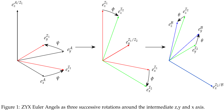
Problem 1 (Characterizations of Rotations)

Euler Angles We have

$$R_{\mathcal{B}}^A(\theta ,\varphi ,\psi )=R_z(\psi )R_y(\varphi )R_x(\theta )$$

and

$$\chi =\left[\begin{array}{c}\theta \\ \varphi \\ \psi \end{array}\right]$$

a)

Used formulas:

Skew-Symmetric Cross Product Matrix Formula

[!Skew-Symmetric Cross Product Matrix Formula]

$[{\omega }_{\mathcal{P}\mathcal{Q}}^{\mathcal{P}}{]}_{\times }={\dot{R}}_Q^{\mathcal{P}}(R_{\mathcal{Q}}^{\mathcal{P}}{)}^T$

Remember Skew-Symmetric Matrix

See Assignment 3 - Kinematics 2

Link to original

Where the Skew-Symmetric Matrix is on the form

Transclude of Skew-Symmetric-Matrix#^36cc79

And the vector is given by

Link to original

We have the following Principal Rotation Matrix for $z,y,x$

Link to original

---

We first find ${\mathcal{R}}_{{\mathcal{I}}_1}^{\mathcal{A}}$, which is a principal rotation matrix around the $z$-axis.

$${\mathcal{R}}_{{\mathcal{I}}_1}^{\mathcal{A}}=\left[\begin{array}{ccc}\cos \psi & -\sin \psi & 0\\ \sin \psi & \cos \psi & 0\\ 0& 0& 1\end{array}\right]$$

Which has the related relative angular velocity, ${\omega }_{{\mathcal{A}\mathcal{I}}_1}^{\mathcal{A}}$.

$$\begin{array}{rl}[{\omega }_{{\mathcal{A}\mathcal{I}}_1}^{\mathcal{A}}{]}_{\times }& ={\dot{\mathcal{R}}}_{{\mathcal{I}}_1}^{\mathcal{A}}({\mathcal{R}}_{{\mathcal{I}}_1}^{\mathcal{A}}{)}^T\\ [{\omega }_{{\mathcal{A}\mathcal{I}}_1}^{\mathcal{A}}{]}_{\times }& =\left[\begin{array}{ccc}-\dot{\psi }\sin \psi & -\dot{\psi }\cos \psi & 0\\ \dot{\psi }\cos \psi & -\dot{\psi }\sin \psi & 0\\ 0& 0& 0\end{array}\right]\left[\begin{array}{ccc}\cos \psi & \sin \psi & 0\\ -\sin \psi & \cos \psi & 0\\ 0& 0& 1\end{array}\right]\\ [{\omega }_{{\mathcal{A}\mathcal{I}}_1}^{\mathcal{A}}{]}_{\times }& =\left[\begin{array}{ccc}0& -\dot{\psi }& 0\\ \dot{\psi }& 0& 0\\ 0& 0& 0\end{array}\right]\end{array}$$

Which means that ${\omega }_{{\mathcal{A}\mathcal{I}}_1}^{\mathcal{A}}=\left[\begin{array}{c}0\\ 0\\ \dot{\psi }\end{array}\right]$

---

We then find ${\mathcal{R}}_{{\mathcal{I}}_2}^{{\mathcal{I}}_1}$, which is a principal rotation matrix around the $y$-axis.

$${\mathcal{R}}_{{\mathcal{I}}_2}^{{\mathcal{I}}_1}=\left[\begin{array}{ccc}\cos \varphi & 0& \sin \varphi \\ 0& 1& 0\\ -\sin \varphi & 0& \cos \varphi \end{array}\right]$$

Which has the related relative angular velocity, ${\omega }_{{\mathcal{I}}_1{\mathcal{I}}_2}^{{\mathcal{I}}_1}=\left[\begin{array}{c}0\\ \dot{\varphi }\\ 0\end{array}\right]$ (by solving the same way).

---

And lastly ${\mathcal{R}}_{\mathcal{B}}^{{\mathcal{I}}_2}$, which is a principal rotation matrix around the $x$-axis.

$${\mathcal{R}}_{\mathcal{B}}^{{\mathcal{I}}_2}=\left[\begin{array}{ccc}1& 0& 0\\ 0& \cos \theta & -\sin \theta \\ 0& \sin \theta & \cos \theta \end{array}\right]$$

Which has the related relative angular velocity, ${\omega }_{{\mathcal{I}}_2\mathcal{B}}^{{\mathcal{I}}_2}=\left[\begin{array}{c}\dot{\theta }\\ 0\\ 0\end{array}\right]$

b)

We want to express ${\omega }_{\mathcal{A}/\mathcal{B}}^{\mathcal{A}}$ as

$${\omega }_{\mathcal{A}/\mathcal{B}}^{\mathcal{A}}=E\dot{\chi }$$

Where $\dot{\chi }={\left[\begin{array}{ccc}\dot{\theta }& \dot{\varphi }& \dot{\psi }\end{array}\right]}^T$.

---

Finding the composite relative angular velocities is the same as the sum

$$\begin{array}{rl}{\omega }_{\mathcal{A}/\mathcal{B}}^{\mathcal{A}}& ={\omega }_{{\mathcal{A}\mathcal{I}}_1}^{\mathcal{A}}+{\omega }_{{\mathcal{I}}_1{\mathcal{I}}_2}^{\mathcal{A}}+{\omega }_{{\mathcal{I}}_2\mathcal{B}}^{\mathcal{A}}\\ & ={\omega }_{{\mathcal{A}\mathcal{I}}_1}^{\mathcal{A}}+{\mathcal{R}}_{{\mathcal{I}}_1}^{\mathcal{A}}{\omega }_{{\mathcal{I}}_1{\mathcal{I}}_2}^{{\mathcal{I}}_1}+{\mathcal{R}}_{{\mathcal{I}}_2}^{\mathcal{A}}{\omega }_{{\mathcal{I}}_2\mathcal{B}}^{{\mathcal{I}}_2}\\ & ={\omega }_{{\mathcal{A}\mathcal{I}}_1}^{\mathcal{A}}+{\mathcal{R}}_{{\mathcal{I}}_1}^{\mathcal{A}}{\omega }_{{\mathcal{I}}_1{\mathcal{I}}_2}^{{\mathcal{I}}_1}+{\mathcal{R}}_{{\mathcal{I}}_1}^{\mathcal{A}}{\mathcal{R}}_{{\mathcal{I}}_2}^{{\mathcal{I}}_1}{\omega }_{{\mathcal{I}}_2\mathcal{B}}^{{\mathcal{I}}_2}\\ & =\left[\begin{array}{ccc}{\mathcal{R}}_{{\mathcal{I}}_1}^{\mathcal{A}}{\mathcal{R}}_{{\mathcal{I}}_2}^{{\mathcal{I}}_1}\left[\begin{array}{c}1\\ 0\\ 0\end{array}\right],& {\mathcal{R}}_{{\mathcal{I}}_1}^{\mathcal{A}}\left[\begin{array}{c}0\\ 1\\ 0\end{array}\right],& \left[\begin{array}{c}0\\ 0\\ 1\end{array}\right]\end{array}\right]\left[\begin{array}{c}\dot{\theta }\\ \dot{\varphi }\\ \dot{\psi }\end{array}\right]\end{array}$$

Which yields

$$\begin{array}{rl}E& =\left[\begin{array}{ccc}{\mathcal{R}}_{{\mathcal{I}}_1}^{\mathcal{A}}{\mathcal{R}}_{{\mathcal{I}}_2}^{{\mathcal{I}}_1}\left[\begin{array}{c}1\\ 0\\ 0\end{array}\right],& {\mathcal{R}}_{{\mathcal{I}}_1}^{\mathcal{A}}\left[\begin{array}{c}0\\ 1\\ 0\end{array}\right],& \left[\begin{array}{c}0\\ 0\\ 1\end{array}\right]\end{array}\right]\\ E& =\left[\begin{array}{ccc}\cos \varphi \cos \psi & -\sin \psi & 0\\ \cos \varphi \sin \psi & \cos \psi & 0\\ -\sin \varphi & 0& 1\end{array}\right]\end{array}$$

Q.E.D

c)

When $\varphi =\frac{\pi }{2}+k\pi ,\forall k\in \mathbb{Z}$, we get the following $E$ matrix.

$$E=\left[\begin{array}{ccc}0& -\sin \psi & 0\\ 0& \cos \psi & 0\\ \pm 1& 0& 1\end{array}\right]$$

The resulting determinant is equal to zero when the bottom left element is both positive and negative. $E$ is therefore singular, and cannot be inverted. Exactly this is the weakness of Euler Angles, and is the reason we choose Angle Axis Representation or Quaternions instead when these situations can arise.

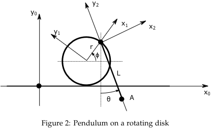
Problem 2 (Pendulum on rotating disk)

Equation $60$

Link to original

---

Equation $77$

Link to original

a)

We want to find the Linear Velocity of point $A$ represented in the $0$-frame, ${\vec{v}}_{A/0}^0$.

We first find ${\vec{v}}_{A/2}^2$.

$$\begin{array}{rl}{\vec{v}}_{A/2}^2& ={\vec{\omega }}_{\theta }^2\times {\vec{r}}_{A/2}^2\\ {\vec{v}}_{A/2}^2& =\left[\begin{array}{c}0\\ 0\\ \dot{\theta }\end{array}\right]\times \left[\begin{array}{c}0\\ -L\\ 0\end{array}\right]\\ {\vec{v}}_{A/2}^2& =\left|\begin{array}{ccc}\vec{i}& \vec{j}& \vec{k}\\ 0& 0& \dot{\theta }\\ 0& -L& 0\end{array}\right|\\ {\vec{v}}_{A/2}^2& =\left[\begin{array}{c}L\dot{\theta }\\ 0\\ 0\end{array}\right]\end{array}$$

We get ${\vec{\omega }}_{\theta }^2=[0,0,\dot{\theta }{]}^T$ since we rotate about the $z$-axis in positive direction

We then find $v_{A/1}^1$

$$\begin{array}{rl}{\vec{v}}_{A/1}^1& ={\vec{v}}_{2/1}^1+{\vec{v}}_{A/2}^1\\ {\vec{v}}_{A/1}^1& =({\vec{\omega }}_{\varphi }^1\times {\vec{r}}_{2/1}^1)+R_2^1{\vec{v}}_{A/2}^2\end{array}$$

Since we can see that $R_2^1=R_z(\theta -\varphi )$, we get

$$\begin{array}{rl}{\vec{v}}_{A/1}^1& =\left[\begin{array}{c}0\\ 0\\ \dot{\varphi }\end{array}\right]\times \left[\begin{array}{c}r\\ 0\\ 0\end{array}\right]+\left[\begin{array}{ccc}\cos (\theta -\varphi )& -\sin (\theta -\varphi )& 0\\ \sin (\theta -\varphi )& \cos (\theta -\varphi )& 0\\ 0& 0& 1\end{array}\right]\left[\begin{array}{c}L\dot{\theta }\\ 0\\ 0\end{array}\right]\\ {\vec{v}}_{A/1}^1& =\left[\begin{array}{c}0\\ r\dot{\varphi }\\ 0\end{array}\right]+\left[\begin{array}{c}L\dot{\theta }\cos (\theta -\varphi )\\ L\dot{\theta }\sin (\theta -\varphi )\\ 0\end{array}\right]\\ {\vec{v}}_{A/1}^1& =\left[\begin{array}{c}L\dot{\theta }\cos (\theta -\varphi )\\ r\dot{\varphi }+L\dot{\theta }\sin (\theta -\varphi )\\ 0\end{array}\right]\end{array}$$

We get ${\vec{\omega }}_{\varphi }^1=[0,0,\dot{\varphi }{]}^T$ since we rotate about the $z$-axis in positive direction

Lastly we find ${\vec{v}}_{A/0}^0$

$$\begin{array}{rl}{\vec{v}}_{A/0}^0& ={\vec{v}}_{1/0}^0+{\vec{v}}_{2/1}^0+{\vec{v}}_{A/2}^0\\ {\vec{v}}_{A/0}^0& ={\vec{v}}_{1/0}^0+{\vec{v}}_{A/1}^0\\ {\vec{v}}_{A/0}^0& =({\vec{\omega }}_{\varphi }^0\times {\vec{r}}_{1/0}^0)+R_1^0{\vec{v}}_{A/1}^1\\ {\vec{v}}_{A/0}^0& =\left[\begin{array}{c}0\\ 0\\ \dot{\varphi }\end{array}\right]\times \left[\begin{array}{c}0\\ r\\ 0\end{array}\right]+R_z(\varphi )\left[\begin{array}{c}L\dot{\theta }\cos (\theta -\varphi )\\ r\dot{\varphi }+L\dot{\theta }\sin (\theta -\varphi )\\ 0\end{array}\right]\\ {\vec{v}}_{A/0}^0& =\left[\begin{array}{c}-r\dot{\varphi }(1+\sin \varphi )+L\dot{\theta }\cos \theta \\ r\dot{\varphi }\cos \varphi +L\dot{\theta }\sin \theta \\ 0\end{array}\right]\end{array}$$

The reason that we have ${\omega }_{\varphi }^0=[0,0,\dot{\varphi }{]}^T$ is still due to rotation around $z$-axis.

b)

We want to find the Linear Acceleration, ${\vec{a}}_A^0$. We do this by derivating term by term.

$$\begin{array}{rl}{\vec{a}}_A^0& =\frac{d}{dt}{\vec{v}}_{A/2}^0\\ {\vec{a}}_A^0& =\left[\begin{array}{c}L(\ddot{\theta }-{\dot{\theta }}^2\sin \theta )-r(\ddot{\varphi }+\ddot{\varphi }\sin \varphi +{\dot{\varphi }}^2\cos \varphi )\\ r(\ddot{\varphi }\cos \varphi -{\dot{\varphi }}^2\sin \varphi )+L(\ddot{\theta }\sin \theta +{\dot{\theta }}^2\cos \theta )\\ 0\end{array}\right]\end{array}$$

I got the answer from WolframAlpha, and did a bit of simplifications.

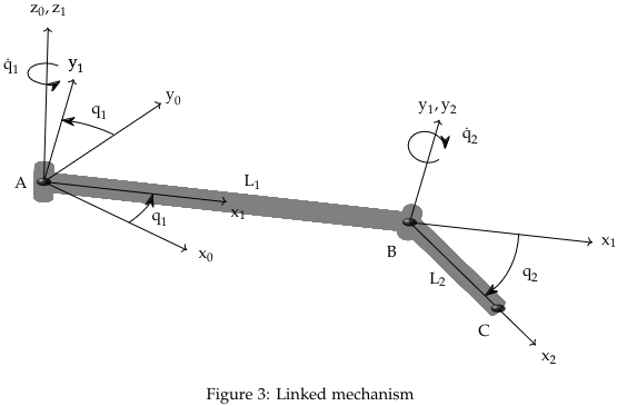
Problem 3 (Linked Mechanism)

a)

We want to find the position of $B$ relative to $A$ in the $0$-frame, $r_{B/A}^0$, and the position of $C$ relative to $A$ in the $0$-frame, $r_{C/A}^0$.

We first find $r_{B/A}^0(q)$

$$\begin{array}{rl}{r}_{B/A}^0(q)& =R_1^0{r}_{B/A}^1\\ r_{B/A}^0(q)& =R_z(q_1)r_{B/A}^1\\ r_{B/A}^0(q)& =\left[\begin{array}{ccc}\cos q_1& -\sin q_1& 0\\ \sin q_1& \cos q_1& 0\\ 0& 0& 1\end{array}\right]\left[\begin{array}{c}{L}_1\\ 0\\ 0\end{array}\right]\\ r_{B/A}^0(q)& =\left[\begin{array}{c}{L}_1\cos q_1\\ L_1\sin q_1\\ 0\end{array}\right]\end{array}$$

We then find $r_{C/A}^0(q)$

$$\begin{array}{rl}{r}_{C/A}^0(q)& =r_{B/A}^0(q)+r_{C/B}^0(q)\\ r_{C/A}^0(q)& =r_{B/A}^0(q)+R_1^0{R}_2^1{r}_{C/B}^2\\ r_{C/A}^0(q)& =r_{B/A}^0(q)+R_z(q_1)R_y(-q_2)r_{C/B}^2\\ r_{C/A}^0(q)& =\left[\begin{array}{c}{L}_1\cos q_1\\ L_1\sin q_1\\ 0\end{array}\right]+\left[\begin{array}{ccc}\cos q_1& -\sin q_1& 0\\ \sin q_1& \cos q_1& 0\\ 0& 0& 1\end{array}\right]\left[\begin{array}{ccc}\cos q_2& 0& -\sin q_2\\ 0& 1& 0\\ \sin q_2& 0& \cos q_2\end{array}\right]\left[\begin{array}{c}{L}_2\\ 0\\ 0\end{array}\right]\\ r_{C/A}^0(q)& =\left[\begin{array}{c}{L}_1\cos q_1+L_2\cos q_1\cos q_2\\ L_1\sin q_1+L_2\sin q_1\cos q_2\\ L_2\sin q_2\end{array}\right]\end{array}$$

Alternatively, in Matlab using the symbolic toolbox

% Define symbolic variables
syms L1 L2 q1 q2 real
 
% Rotation matrices,@(angle) creates an anonymous function
Rz = @(angle) [cos(angle) -sin(angle) 0; sin(angle) cos(angle) 0; 0 0 1];
Ry = @(angle) [cos(angle) 0 sin(angle); 0 1 0; -sin(angle) 0 cos(angle)];
 
% Position vector from A to B in frame 0
r0_B_A = Rz(q1) * [L1; 0; 0];
 
% Position vector from B to C in frame 0
r0_C_B = Rz(q1) * Ry(-q2) * [L2; 0; 0];
 
% Position vector from A to C in frame 0
r0_C_A = r0_B_A + r0_C_B;
 
% Output the results
r0_B_A = simplify(r0_B_A)
r0_C_A = simplify(r0_C_A)

b)

Keeping the code from a), we can extend our script to also give us angular velocity

% Define symbolic variables for the angular velocities
syms q1_dot q2_dot real
 
% Define the angular velocity of AB in the global frame
omega_AB = [0; 0; q1_dot];
 
% Calculate the angular velocity of BC in the local frame and rotate to global frame
omega_BC_local = [0; q2_dot; 0];
omega_BC_global = Rz(q1) * omega_BC_local;
 
% The total angular velocity of BC in the global frame is the sum of omega_AB and the rotated omega_BC_local
omega_BC = omega_AB + omega_BC_global;
 
% Output the results
omega_AB = simplify(omega_AB)
omega_BC = simplify(omega_BC)

Which gives us

$$\begin{array}{r}{\vec{\omega }}_{AB/0}^0=\left[\begin{array}{c}0\\ 0\\ {\dot{q}}_2\end{array}\right]\end{array}$$

And

$${\vec{\omega }}_{BC/0}^0=\left[\begin{array}{c}-{\dot{q}}_2\sin q_1\\ {\dot{q}}_2\cos q_1\\ {\dot{q}}_1\end{array}\right]$$

c)

Keeping the code from b) and c), and extending it lets us also find the Linear Velocity

% Define symbolic variables
syms L1 L2 q1 q2 q1_dot q2_dot real
 
% Position vectors from A to B and from B to C in frame 0
r0_B_A = [L1*cos(q1); L1*sin(q1); 0];
r0_C_B = [L2*cos(q1+q2); L2*sin(q1+q2); 0];
 
% Angular velocities in frame 0
omega_AB = [0; 0; q1_dot];
omega_BC = [0; 0; q1_dot + q2_dot];
 
% Calculate the linear velocity of point B
v_B = cross(omega_AB, r0_B_A);
 
% Calculate the linear velocity of point C
v_C = v_B + cross(omega_BC, r0_C_B - r0_B_A);
 
% Output the results
v_B = simplify(v_B)
v_C = simplify(v_C)

Which gives us

$${\vec{v}}_{B/0}^0=\left[\begin{array}{c}-L_1{\dot{q}}_1\sin q_1\\ L_1{\dot{q}}_1\cos q_1\\ 0\end{array}\right]$$

And

$${\vec{v}}_{C/0}^0=\left[\begin{array}{c}-({\dot{q}}_1+{\dot{q}}_2)(L_2\sin (q_1+q_2)-L_1\sin q_1-L_1{\dot{q}}_1\sin q_1)\\ (L_2\cos (q_1+q_2)-L_1\cos q_1)({\dot{q}}_1+{\dot{q}}_2)+L_1{\dot{q}}_1\cos q_1\\ 0\end{array}\right]$$

d)

We want to express the linear velocity of the point $C$ as $v_{C/0}=J(q)\dot{q}$, with a Jacobian matrix $J$. This can be done in the following matlab script

% Define symbolic variables
syms L1 L2 q1 q2 q1_dot q2_dot real
% Position vector of point C from A
r0_C_A = [L1*cos(q1) + L2*cos(q1 + q2); L1*sin(q1) + L2*sin(q1 + q2); 0];
% Compute the Jacobian matrix
J = [diff(r0_C_A, q1), diff(r0_C_A, q2)];
% The vector of joint velocities
q_dot = [q1_dot; q2_dot];
% The linear velocity of point C
v_C = J * q_dot;
% Simplify the expression
v_C = simplify(v_C);
% Display the Jacobian matrix and the linear velocity of point C
J
v_C

Which yields

$$J=\left[\begin{array}{cc}-L_2\sin (q_1+q_2)-L_1\sin q_1& -L_2\sin (q_1+q_2)\\ L_2\cos (q_1+q_2)+L_1\cos q_1& L_2\cos (q_1+q_2)\\ 0& 0\end{array}\right]$$

The Entire Matlab Script For Problem 3

 Angular Velocity
% Define symbolic variables for the angular velocities
syms q1_dot q2_dot real
 
% Define the angular velocity of AB in the global frame
omega_AB = [0; 0; q1_dot];
 
% Calculate the angular velocity of BC in the local frame and rotate to global frame
omega_BC_local = [0; q2_dot; 0];
omega_BC_global = Rz(q1) * omega_BC_local;
 
% The total angular velocity of BC in the global frame is the sum of omega_AB and the rotated omega_BC_local
omega_BC = omega_AB + omega_BC_global;
 
% Output the results
omega_AB = simplify(omega_AB)
omega_BC = simplify(omega_BC)
 
 
 Linear Velocity on Jacobian form
% Define symbolic variables
syms L1 L2 q1 q2 q1_dot q2_dot real
% Position vector of point C from A
r0_C_A = [L1*cos(q1) + L2*cos(q1 + q2); L1*sin(q1) + L2*sin(q1 + q2); 0];
% Compute the Jacobian matrix
J = [diff(r0_C_A, q1), diff(r0_C_A, q2)];
% The vector of joint velocities
q_dot = [q1_dot; q2_dot];
% The linear velocity of point C
v_C = J * q_dot;
% Simplify the expression
v_C = simplify(v_C);
% Display the Jacobian matrix and the linear velocity of point C
J
v_C