We add an additional term that gives us information about the deviation between output and estimated output
Where , and is an estimator gain which we choose to make up for modeling errors and disturbances, and send with desired convergence rate.
\dot{e}&=\dot{x} - \dot{\hat{x}} \\ \dot{e} &= Ax+Bu-[A\hat{x}+Bu+L(y-\hat{y}] \\ \dot{e} &= A(x-\dot{x})-L(C(x-\hat{x})+n) \\ \dot{e} &=(A-LC)e-Ln \end{align}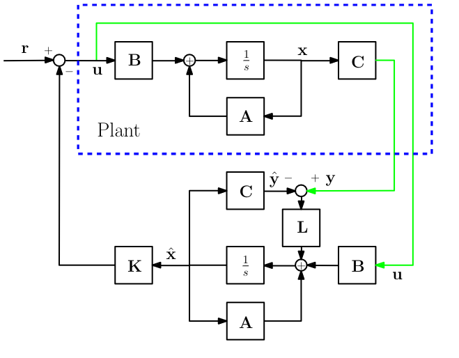
We can choose poles in by selecting a Real constant matrix, , if and only if and are observable.
This means that, by modifying L, we can make the new system stable, even if the original system was unstable
THE ERROR DYNAMICS SHOULD BE FASTER THAN THE PLANT ITSELF: x2 -20 → VI må ha poler som er høyere enn system i observatoren.
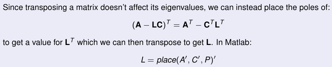
Pole Placement In Matlab- Luenberger Observer
Given that we want to place the poles of the matrix:
we can use the matlab function