Design of Digital Filters - FIR, IIR

Resources: page=680

Ideal filters are non-causal and infinite lasting. Example with an ideal low pass filter:

$$\begin{array}{rl}{H}_l(\omega )& =\{\begin{array}{ll}1,& |\omega |\le {\omega }_c\\ 0,& {\omega }_c<\omega \le \pi \end{array}\\ h_l[n]& =\{\begin{array}{ll}\frac{{\omega }_c}{\pi },& n=0\\ \frac{{\omega }_c}{\pi }\frac{\sin ({\omega }_{c}n)}{{\omega }_{c}n},& n\ne 0\end{array}\end{array}$$

\usepackage{pgfplots}
\pgfplotsset{compat=1.16}
\begin{document}
\begin{tikzpicture}
\begin{axis}
[
ymax = 0.3,
clip = false,
ycomb,
axis lines = middle,
xlabel = $n$,
ylabel = {h[n]},
title = {Ideal discrete low pass filter}
]
\addplot
[ 
 color = red,
 samples=50, 
 domain=-20:20,
 mark=o,
 ]{pi/4/pi*(sin(deg(pi/4*x)))/(pi/4*x)} 
 node[right, pos=1]{$f(x)=pi/4/pi*(sin(deg(pi/4*x)))/(pi/4*x)$};
\end{axis}
\end{tikzpicture}
\end{document}

We want causal linear-phase filters which needs approximations. The filter must not “spill” into the next frequency band.

FIR vs IIR

FIR:

• Always stable
• Can achieve exactly Linear Phase
• Easily designed with linear methods
• Easy to implement

IIR:

• Fewer parameters (low filter order)
• Less memory
• Low delay
• Lower computational complexity
• Typically designed by transforming an analog filter design

FIR

Goal - Find $b_k$: $H(z)={\sum }_{k=0}^{M-1}{b}_k{z}^{-k}$ → $y[n]={\sum }_{k=0}^{M-1}{b}_{k}x[n-k]$

Design Using Windows

Using this method, we begin with the desired frequency response specification, $H_d(\omega )$, and then determine the corresponding unit sample response $h_d[n]$.

$$\begin{array}{rl}{H}_d(\omega )& \stackrel{\mathcal{F}}{\to }{h}_d[n]\\ H_d(\omega )& =\sum _{n=0}^{\infty }{h}_d[n]e^{-j\omega n}\end{array}$$

We are looking at Finite Impulse Response, therefore we look at $n=M-1$. This can we done with a window function like this

$$w(n)=\{\begin{array}{ll}1,& n=0,1,\dots ,M-1\\ 0,& \text{ce}otherwise\end{array}$$

And looking at the Fourier transform gives us

$$W(\omega )=\sum _{n=0}^{M-1}{e}^{-j\omega n}=\cdots =e^{-jw(M-1)/2}\frac{\sin (\omega M/2)}{\sin (\omega /2)}$$

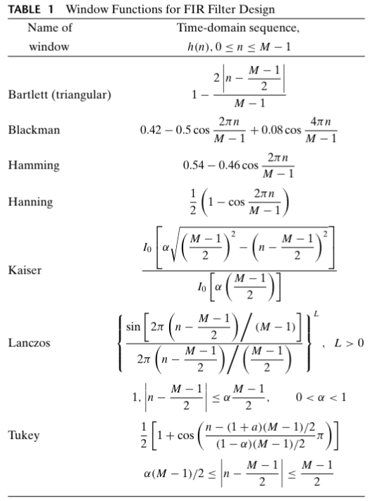
We also have tons of other window functions

IIR

Goal - Find $a_k$ and $b_k$: $H(z)=\frac{{\sum }_{k=0}^{M-1}{b}_k{z}^{-k}}{1+{\sum }_{k=1}^N{a}_k{z}^{-k}}$ → $y[n]=-{\sum }_{k=1}^N{a}_k{z}^{-k}+{\sum }_{k=0}^{M-1}{b}_{k}x[n-k]$

\usepackage{pgfplots}
\pgfplotsset{compat=1.16}
\begin{document}
\begin{tikzpicture}
\begin{axis}
[
clip = false,
axis lines = middle,
xlabel = $x$,
ylabel = $y$,
title = {edvard er homo}
]
\addplot
[ 
 color = blue,
 samples=50, 
 domain=-2:2,
 ]{x²} 
 node[right, pos=1]{$f(x)=x²$};
\end{axis}
\end{tikzpicture}
\end{document}