Exercise 4 - Quadratic Programming

Lecture 6&7 - Quadratic Programming

Problem 1 (50%) Quadratic Programming

a)

Given a Quadratic Programming Problem on Standard Form

Link to original

This is a convex problem if the Hessian of $G$ is a Positive-Semidefinite Matrix. If the Hessian of $G$ is a Positive-Definite Matrix matrix, the QP is strictly convex.

Convexity is important due to many factors, if the QP is convex then:

• Any local solution is a global solution
• Algorithms are more efficient, and can often guarantee convergence.

b)

If $Z^{T}GZ\ge 0$ instead of $Z^{T}GZ>0$ as in the proof of theorem 16.2 in page=475, we can only say that we have a local minimizer, but that it is not strict. We can see that in the last equation of the proof

$$q(x)=\frac{1}{2}{u}^T{Z}^{T}GZu+q(x^{\ast })$$

Since $Z^{T}GZ$ can be $0$, there is a possibility that $q(x)=q(x^{\ast })$, instead of guaranteeing that $q(x)>q(x^{\ast })$.

c)

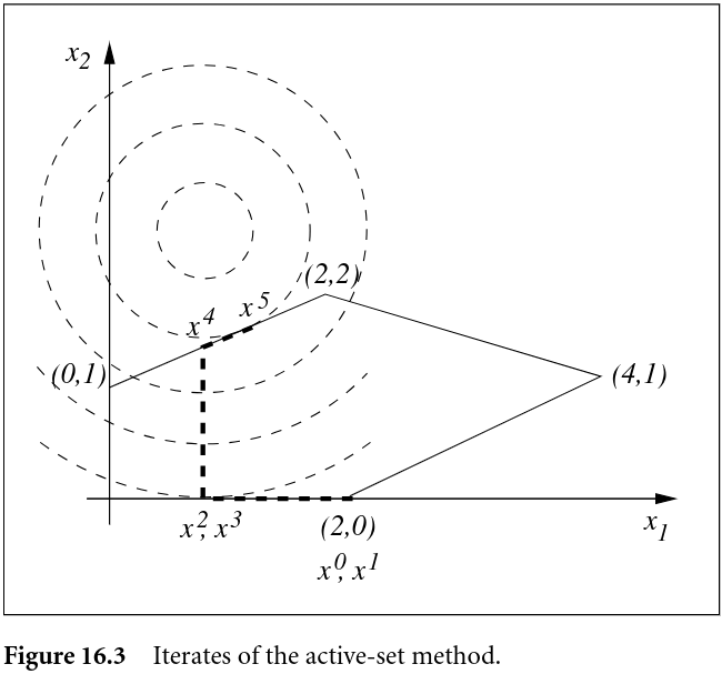
page=497 Algorithm 16.3 is called the Active-Set Method for Convex QP. If we change the starting point to be $x=[2,0{]}^T$, and we assume that the constraint $-x_1+2x_2+2\ge 0$ is active (aka ${\mathcal{W}}_0=\{3\}$), then the algorithm would do as follows.

---

We have the following problem

$$\underset{x\in {\mathbb{R}}^n}{\min }q(x)=(x_1-1{)}^2+(x_2-2.5{)}^{2}s.t.\{\begin{array}{ll}{x}_1-2x_2+2& \ge 0\\ -x_1-2x_2+6& \ge 0\\ -x_1+2x_2+2& \ge 0\\ x_1,x_2& \ge 0\end{array}$$

Rewriting this into a Quadratic Programming Problem on Standard Form

Link to original

We get

$$\begin{array}{rl}G& =\left[\begin{array}{cc}2& 0\\ 0& 2\end{array}\right],c^T=\left[\begin{array}{cc}-2& 5\end{array}\right],A=\left[\begin{array}{cc}1& -2\\ -1& -2\\ -1& 2\\ 1& 0\\ 0& 1\end{array}\right],b=\left[\begin{array}{c}-2\\ -6\\ -2\\ 0\\ 0\end{array}\right]\end{array}$$

Where we only have inequality constraints, $\{1,2,3,4,5\}\in \mathcal{I}$. The constant value in the objective function which is $7.25$ (which we ignore) does not change the solution.

…

d) Duality for Nonlinear Programming

As seen in c), we know that we can write the QP on standard form, and we know the values for $G$, $A$, $c$ and $b$.

We start by finding the Lagrangian

$$\begin{array}{rl}\mathcal{L}(x,\lambda )& =\frac{1}{2}{x}^{T}Gx+x^{T}c-{\lambda }^T(Ax-b)\end{array}$$

Then, the dual objective function, $q$, is given by

$$\begin{array}{rl}q(\lambda )& =\underset{x}{\inf }\mathcal{L}(x,\lambda )\\ q(\lambda )& =\underset{x}{\inf }\frac{1}{2}{x}^{T}Gx+x^{T}c-{\lambda }^T(Ax-b)\end{array}$$

The Infimum of a strictly convex quadratic function ($G>0$) with respect to $x$ is

$$\begin{array}{rlr}{\nabla }_x\mathcal{L}(x,\lambda )& =0& \\ {\nabla }_x\mathcal{L}(x,\lambda )& =Gx+c-A^T\lambda =0& \text{Since }G=G^T\end{array}$$

Solving for $x$, and putting this into the function for the Lagrangian, $\mathcal{L}(x(\lambda ),\lambda )=q(\lambda )$, gives us

$$q(\lambda )=-\frac{1}{2}(A^T\lambda -c{)}^T{G}^{-1}(A^T\lambda -c)+{\lambda }^{T}b$$

Thus giving us the dual problem

$$\underset{\lambda }{\max }-\frac{1}{2}(A^T\lambda -c{)}^T{G}^{-1}(A^T\lambda -c)+{\lambda }^{T}bs.t.\lambda \ge 0$$

e) Weak Duality

From theorem 12.11 in the book about Weak Duality, we know that

Link to original

Which we can rewrite as

$$f(\bar{x})-f(x^{\ast })\le f(\bar{x})-q(\bar{\lambda })$$

Thus giving us an over estimate when the optimal point is unknown.

Problem 2 (50%) Production Planning and Quadratic Programming

We are given the following optimization problem

$$\underset{x}{\max }(3-0.4x_1)x_1+(2-0.2x_2)x_{2}s.t.\{\begin{array}{ll}2x_1+x_2& \le 8\\ x_1+3x_2& \le 15\\ x_1,x_2& \ge 0\end{array}$$

Where

$$\begin{array}{rl}{x}_1& :\text{The production of product A}\\ x_2& :\text{The production of product B}\end{array}$$

a)

Formulating this as a minimization problem can be done the following way

$$\underset{x}{\min }-(3-0.4x_1)x_1-(2-0.2x_2)x_{2}s.t.\{\begin{array}{ll}-2x_1-x_2& \ge -8\\ -x_1-3x_2& \ge -15\\ x_1,x_2& \ge 0\end{array}$$

We can put this on standard form

Link to original

By setting the following matrices

$$\begin{array}{rl}G& =\left[\begin{array}{cc}0.8& 0\\ 0& 0.4\end{array}\right],c=\left[\begin{array}{c}-3\\ -2\end{array}\right]\end{array}$$

b)

The following Matlab script generated the figure below

% Define the range for x1 and x2
x1 = linspace(0, 10, 400);
x2 = linspace(0, 10, 400);
 
% Create a meshgrid for plotting
[X1, X2] = meshgrid(x1, x2);
 
% Calculate the objective function value over the grid
Z = -(3-0.4*X1).*X1 - (2-0.2*X2).*X2;
 
% Plot the contour of the objective function
figure;
contour(X1, X2, Z, 50); % Adjust the number of contours as needed
hold on;
xlabel('x_1');
ylabel('x_2');
title('Contour Plot with Constraints');
 
% Plot the constraints
% -2*x1 - x2 >= -8 -> x2 <= -2*x1 + 8
% -x1 - 3*x2 >= -15 -> x2 <= -1/3*x1 + 5
f1 = @(x1) -2*x1 + 8;
f2 = @(x1) -1/3*x1 + 5;
fplot(f1, [0,10], 'r', 'LineWidth', 2);
fplot(f2, [0,10], 'b', 'LineWidth', 2);
 
% Legend and grid
legend('Objective Function', 'Constraint 1', 'Constraint 2', 'Location', 'BestOutside');
grid on;
hold off;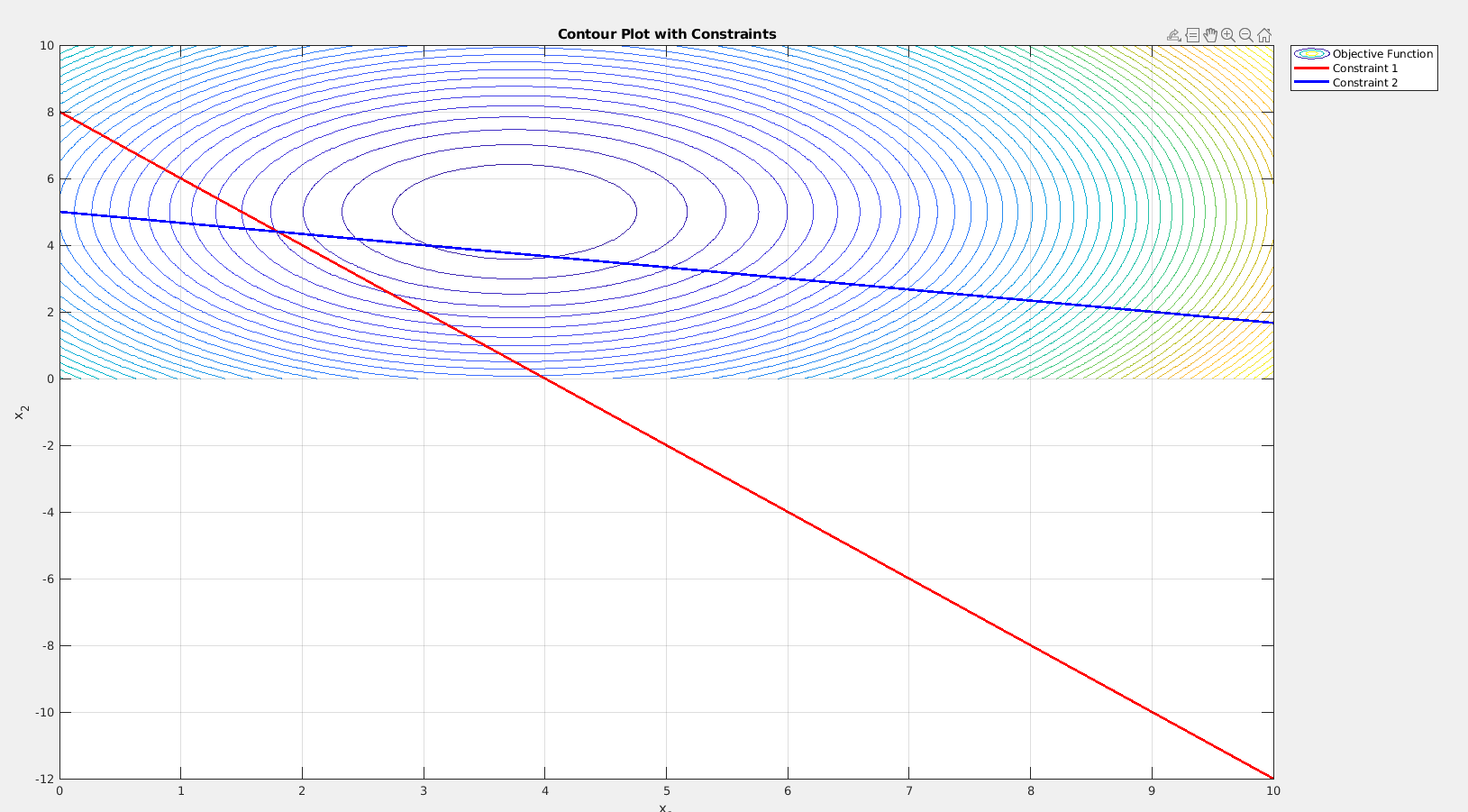

c)

Changing the follow values in the Matlab script

% Objective function
G = [
    0.8 0;
    0   0.4;
    ];
c = [-3; -2];
 
% Constraints
A = [
    -2 -1;
    -1 -3
    ];
b = [-8; -15];

Gives me

Optimization terminated successfully.
Iteration sequence:
         0         0    1.2586    1.8000    3.7500
         0         0    3.7757    4.4000    5.0000

Solution:
    3.7500
    5.0000

The solution is not at a point of intersection between constraints, and no constraints are active.

d)

Active-Set Method for Convex QP We start at a (random really) feasible point, in this case $(0,0)$. Not an optimal point, goes to the next. Etc…

e)

The solution we found in this task has no active constraint, but a LP will always have the solution on a point of intersection. This is quite logical, as the extreme point might be in the middle of the feasible set, but for a LP you can always move to decrease the objective function.