Exercise 1 - The KKT Conditions

TTK4135 - Optimalisering og regulering

Problem 1 (25%)

page=335

---

Given the following problem

$$\text{min}{x}_1+2x_2\text{s.t.}2-x_1^2-x_2^2\ge 0,x_2\ge 0$$

a) By inspection, we can see that the optimal point is given by

$$x^{\ast }=\left[\begin{array}{c}-\sqrt{2}\\ 0\end{array}\right]$$

Since we need to find the minimal point on a circle, where $x_2$ must be greater than zero.

b) From the definition of the Lagrangian we know that it is given by

Link to original

For this problem it is therefore given by (where $\mathcal{I}=\{1,2\}$, and $\mathcal{E}=Ø$)

$$\begin{array}{rl}\mathcal{L}(x,\lambda )& =x_1+2x_2-{\lambda }_1{c}_1(x)-{\lambda }_2{c}_2(x)\\ \mathcal{L}(x,\lambda )& =x_1+2x_2-{\lambda }_1(2-x_1^2-x_2^2)-{\lambda }_2{x}_2\end{array}$$

From the KKT (Karush–Kuhn–Tucker) Conditions, we find

$$\begin{array}{rl}{\nabla }_x\mathcal{L}(x^{\ast },{\lambda }^{\ast })& =0,{\lambda }^{\ast }\ge 0\\ {\nabla }_x\mathcal{L}(x^{\ast },{\lambda }^{\ast })& =\left[\begin{array}{c}1+2{\lambda }_1^{\ast }{x}_1^{\ast }\\ 2+2{\lambda }_1^{\ast }{x}_2^{\ast }-{\lambda }_2\end{array}\right]\end{array}$$

For $x^{\ast }=\left[\begin{array}{c}-\sqrt{2}\\ 0\end{array}\right]$, we get ${\lambda }^{\ast }=\left[\begin{array}{c}\frac{1}{2\sqrt{2}}\\ 2\end{array}\right]$. Since ${\lambda }^{\ast }\ge 0$ the KKT conditions are satisfied at this optimal point.

c) We calculate the gradients of the constrains and the objective function at the solution

$$\begin{array}{rl}{\nabla }_{x}f(x){|}_{x=x^{\ast }}=\left[\begin{array}{c}1\\ 2\end{array}\right]{|}_{x=x^{\ast }}& =\left[\begin{array}{c}1\\ 2\end{array}\right]\\ {\nabla }_x{c}_1(x){|}_{x=x^{\ast }}=\left[\begin{array}{c}-2x_1\\ -2x_2\end{array}\right]{|}_{x=x^{\ast }}& =\left[\begin{array}{c}2\sqrt{2}\\ 0\end{array}\right]\\ {\nabla }_x{c}_2(x){|}_{x=x^{\ast }}=\left[\begin{array}{c}0\\ 1\end{array}\right]{|}_{x=x^{\ast }}& =\left[\begin{array}{c}0\\ 1\end{array}\right]\end{array}$$

d) According to the KKT (Karush–Kuhn–Tucker) Conditions we need the Lagrange multipliers to be positive to satisfy the KKT conditions.

The complementary condition is also called complementary slackness.

Link to original

e) Convex Objective Function

• The objective function is convex since it is a linear function
• The feasible set is convex it is concave Since both the objective function and the feasible set is convex, this is a convex problem.

Problem 2 (30%)

page=330

---

Given the following problem

$$\text{min}2x_1+x_2\text{s.t.}{x}_1^2+x_2^2-2=0$$

Where

$$\begin{array}{rl}f(x)=2x_1+x_2& ,c_1(x)=x_1^2+x_2^2-2\\ \mathcal{I}=Ø& ,\mathcal{E}=\{1\}\end{array}$$

a) From the constraint we can see that the feasible set for this problem is the boundary of a circle of radius $r=\sqrt{2}$ centered at the origin.

Finding the extreme points means finding when ${\nabla }_x\mathcal{L}(x^{\ast },{\lambda }^{\ast })=0$.

$$\begin{array}{rl}\mathcal{L}(x,\lambda )& =f-{\lambda }_1{c}_1\\ & \downarrow \\ {\nabla }_x\mathcal{L}(x^{\ast },{\lambda }^{\ast })& =\left[\begin{array}{c}2\\ 1\end{array}\right]-{\lambda }_1^{\ast }\left[\begin{array}{c}2x_1^{\ast }\\ 2x_2^{\ast }\end{array}\right]=0\\ & \downarrow \\ x^{\ast }& =\left[\begin{array}{c}\frac{1}{{\lambda }_1^{\ast }}\\ \frac{1}{2{\lambda }_1^{\ast }}\end{array}\right]\end{array}$$

Combining this with $x_1^2+x_2^2-2=0$ we solve the system of equations and get the following extreme points

$$x^{\ast }=\pm \left[\begin{array}{c}2\sqrt{\frac{2}{5}}\\ \sqrt{\frac{2}{5}}\end{array}\right]$$

b) From the KKT conditions

The complementary condition is also called complementary slackness.

Link to original

We only need to check the second condition in this case.

$$\begin{array}{rl}{c}_1(x^{\ast })& ={\left(\pm 2\sqrt{\frac{2}{5}}\right)}^2+{\left(\pm \sqrt{\frac{2}{5}}\right)}^2-2\\ c_1(x^{\ast })& =4\frac{2}{5}+\frac{2}{5}-2=0\end{array}$$

Meaning that the KKT conditions at these points are satisfied.

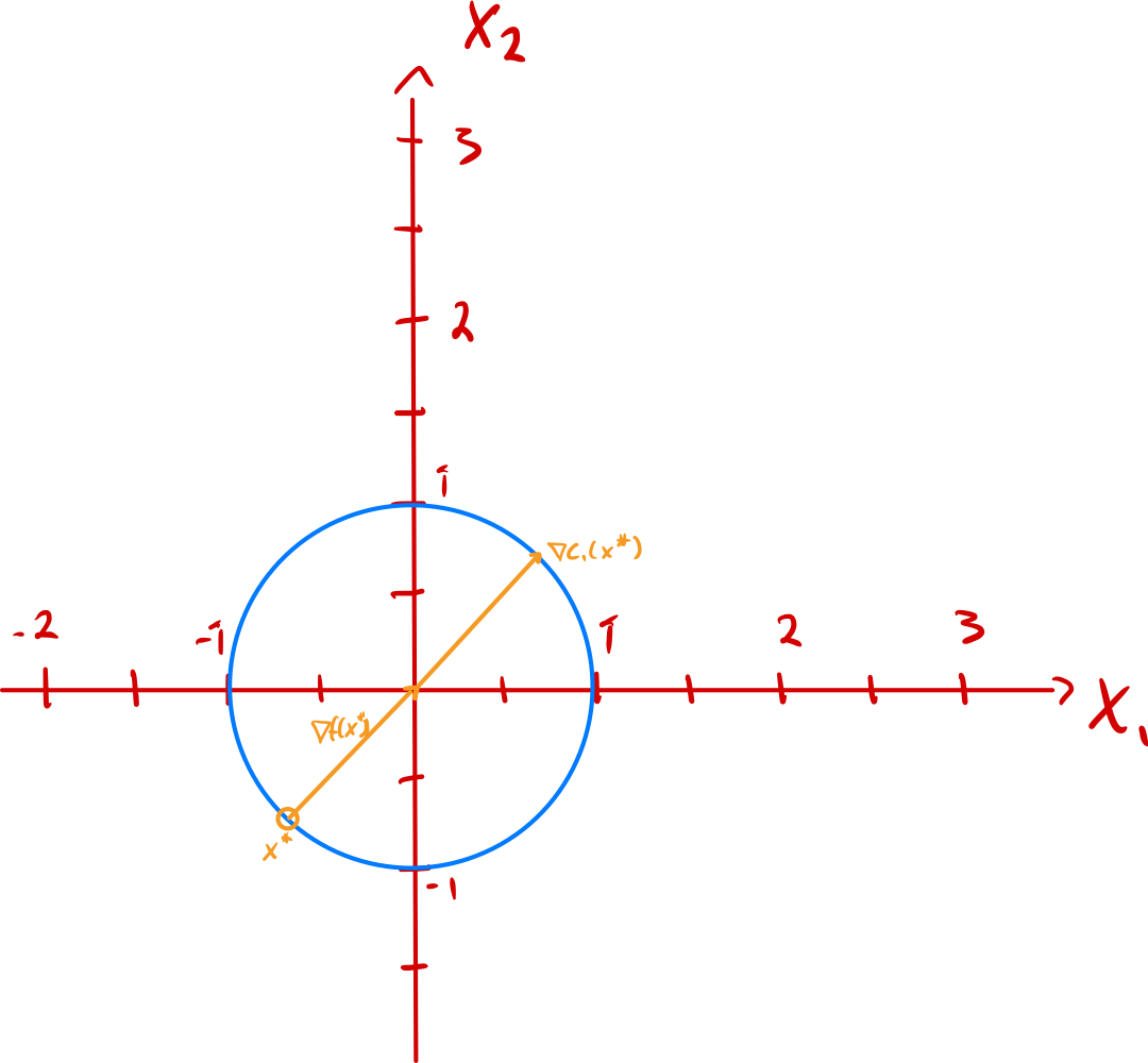
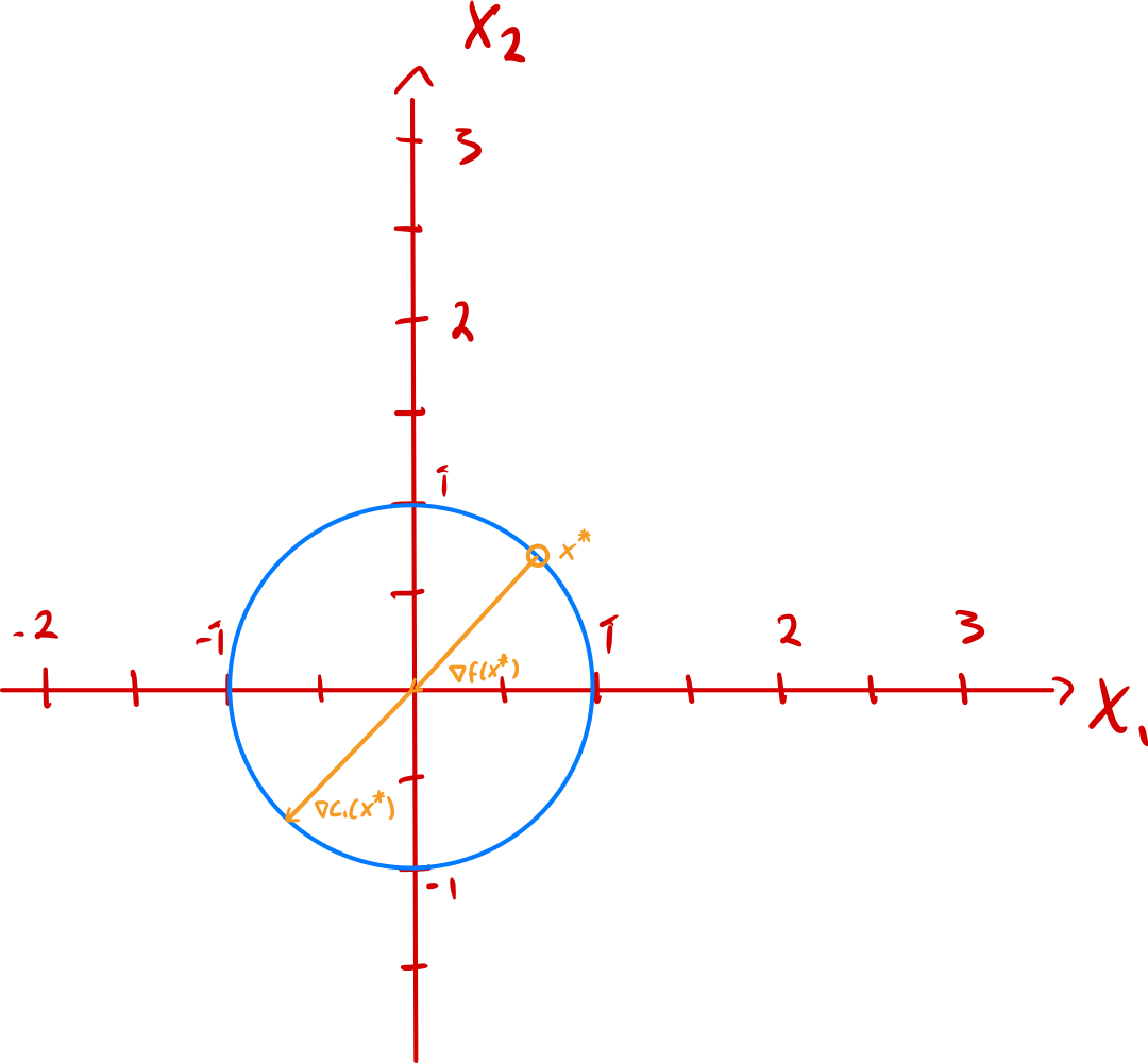
c) Calculating the gradients gives us

$$\nabla c_1(x^{\ast })=\left[\begin{array}{c}2x_1^{\ast }\\ 2x_2^{\ast }\end{array}\right]=\pm \left[\begin{array}{c}\frac{4\sqrt{2}}{\sqrt{5}}\\ \frac{2\sqrt{2}}{\sqrt{5}}\end{array}\right]$$

and

$${\nabla }_{x}f(x^{\ast })=\left[\begin{array}{c}2\\ 1\end{array}\right]$$

Which gives us this for the lower point 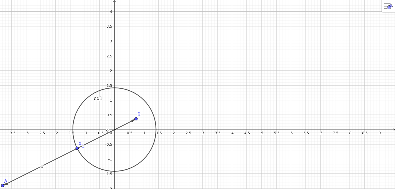Similar results for the other extreme point, but i didn’t plot it.

d) This was calculated in a)

$${\lambda }^{\ast }=\pm \frac{\sqrt{10}}{4}$$

e) We find the second order derivative of the Lagrangian

$$\begin{array}{rl}{\nabla }_{xx}^2\mathcal{L}(x,\lambda ){|}_{x=x^{\ast },\lambda ={\lambda }^{\ast }}& =\left[\begin{array}{cc}\frac{\partial }{\partial x_1}2-2{\lambda }_1{x}_1& \frac{\partial }{\partial x_2}2-2{\lambda }_1{x}_1\\ \frac{\partial }{\partial x_1}2-2{\lambda }_1{x}_2& \frac{\partial }{\partial x_2}2-2{\lambda }_1{x}_2\end{array}\right]{|}_{x=x^{\ast },\lambda ={\lambda }^{\ast }}\\ {\nabla }_{xx}^2\mathcal{L}(x,\lambda ){|}_{x=x^{\ast },\lambda ={\lambda }^{\ast }}& =\left[\begin{array}{cc}-2{\lambda }_1& 0\\ 0& -2{\lambda }_1\end{array}\right]{|}_{x=x^{\ast },\lambda ={\lambda }^{\ast }}\\ {\nabla }_{xx}^2\mathcal{L}(x^{\ast },{\lambda }^{\ast })& =\left[\begin{array}{cc}\frac{\sqrt{10}}{2}& 0\\ 0& \frac{\sqrt{10}}{2}\end{array}\right]>0\end{array}$$

Since this holds (though only for ${\lambda }^{\ast }=-\frac{\sqrt{10}}{4}$), then it follows that

$$w^T{\nabla }_{xx}^2\mathcal{L}(x^{\ast },{\lambda }^{\ast })w>0$$

Also holds for all $w\in \mathcal{C}(x^{\ast },{\lambda }^{\ast }),w\ne 0$, meaning that $x^{\ast }=-{\left[\begin{array}{cc}2\sqrt{\frac{2}{5}}& \sqrt{\frac{2}{5}}\end{array}\right]}^T$ is a strict local solution. (Theorem 12.6).

f) The feasible set is not convex since the equality constraint is not linear. The problem is therefore also not convex.

Problem 3 (20%) - 12.19

page=376

---

Consider the optimization problem

$$\underset{x\in {\mathbb{R}}^2}{\min }f(x)=-2x_1+x_{2}s.t.\{\begin{array}{ll}(1-x_1{)}^3-x_2& \ge 0\\ z_2+0.25x_1-1& \ge 0\end{array}$$

The optimal solution is $x^{\ast }=(0,1{)}^T$, where both constraints are active.

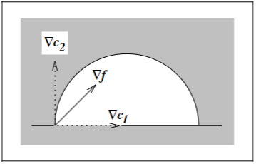
a) Linear Independence Constraint Qualification] The gradients of the active constraints that are active at the optimal solution are

$$\begin{array}{rl}\nabla c_1(x^{\ast })=\left[\begin{array}{c}-3(1-x_1{)}^2\\ -1\end{array}\right]{|}_{x=x^{\ast }}& =\left[\begin{array}{c}-3\\ -1\end{array}\right]\\ \nabla c_2(x^{\ast })={\left[\begin{array}{c}0.5x_1\\ 1\end{array}\right]}_{x=x^{\ast }}& =\left[\begin{array}{c}0\\ 1\end{array}\right]\end{array}$$

Since the vectors are linearly independent, LICQ holds.

b) We find the gradient of the Lagrangian

$${\nabla }_x\mathcal{L}(x,\lambda ){|}_{x=x^{\ast },\lambda ={\lambda }^{\ast }}=\left[\begin{array}{c}-2+3{\lambda }_1(1-x_1{)}^2-0.5{\lambda }_2{x}_1\\ 1+{\lambda }_1-{\lambda }_2\end{array}\right]{|}_{x=x^{\ast },\lambda ={\lambda }^{\ast }}$$

Setting it equal to zero gives us the solution for ${\lambda }^{\ast }$

$$\begin{array}{rl}{\nabla }_x\mathcal{L}(x,\lambda )& {|}_{x=x^{\ast },\lambda ={\lambda }^{\ast }}=0\\ & \downarrow \\ {\lambda }^{\ast }& =\left[\begin{array}{c}\frac{2}{3}\\ \frac{5}{3}\end{array}\right]\end{array}$$

From the KKT conditions, we can see that they are all satisfied.

The complementary condition is also called complementary slackness.

Link to original

c) We want to find The Set of Linearized Feasible Directions, $\mathcal{F}(x)$, , and the Critical Cone, $\mathcal{C}(x,\lambda )$, at the optimum, $x=x^{\ast }$ and $\lambda ={\lambda }^{\ast }$.

We first find $\mathcal{F}(x)$ from the definition

Link to original

Since we have two inequality constraint, where both are active, and no equality constraints we get $\mathcal{A}(x^{\ast })\cap \mathcal{I}=\{1,2\}$. We get the following set of equations for finding $d^T$

$$\begin{array}{rl}1.d^T\nabla c_1(x^{\ast })& \ge 0\\ 2.d^T\nabla c_2(x^{\ast })& \ge 0\end{array}$$

We set $d=\left[\begin{array}{c}{d}_1\\ d_2\end{array}\right]$

$$\begin{array}{rl}1.\left[\begin{array}{cc}{d}_1& d_2\end{array}\right]\left[\begin{array}{c}-3\\ -1\end{array}\right]& \ge 0\\ -3d_1-d_2& \ge 0\\ 2.\left[\begin{array}{cc}{d}_1& d_2\end{array}\right]\left[\begin{array}{c}0\\ 1\end{array}\right]& \ge 0\\ d_2& \ge 0\end{array}$$

Meaning that

$$\mathcal{F}(x^{\ast })=\left\{d|d_1\le -\frac{1}{3}{d}_2\cap d_2\ge 0\right\}$$

Secondly we find $\mathcal{C}(x^{\ast },{\lambda }^{\ast })$ from the definition

Link to original

We already know ${\lambda }^{\ast }=\left[\begin{array}{c}\frac{2}{3}\\ \frac{5}{3}\end{array}\right]$, and $x^{\ast }$, giving us and almost identical set of equations as when finding $\mathcal{F}$ (since ${\lambda }_{{}_i}^{\ast }>0$)

$$\begin{array}{rl}1.\nabla c_1(x^{\ast }{)}^{T}w& =0\\ -3w_1-w_2& =0\\ 2.\nabla c_2(x^{\ast }{)}^{T}w& =0\\ w_2=0& \end{array}$$

Giving us $w_1=w_2=0$. The critical cone is therefore

$$\mathcal{C}(x^{\ast },{\lambda }^{\ast })=\{\left[\begin{array}{c}0\\ 0\end{array}\right]\}$$

d)

1. The Second-Order Necessary Conditions (SONC) is given by

   Link to original

   Since we found $w$ to be $\vec{0}$ in the last task, this condition is satisified

2. The Second-Order Sufficient Condition (SOSC) is given by

   Second-Order Sufficient Condition (SOSC)

   page=355

   ---

   Suppose that for some feasible point $x^{\ast }\in {\mathbb{R}}^n$ there is a Lagrange multiplier vector ${\lambda }^{\ast }$ such that the KKT (Karush–Kuhn–Tucker) Conditions are satisfied. Suppose also that

   $$w^T{\nabla }_{xx}^2\mathcal{L}(x^{\ast },{\lambda }^{\ast })w>0,\forall w\in \mathcal{C}(x^{\ast },{\lambda }^{\ast }),w\ne 0$$

   Then $x^{\ast }$ is a strict local solution.

   Link to original

   We have already found that these satisfy the KKT (Karush–Kuhn–Tucker) Conditions. Since $w=\vec{0}$, but this condition does not consider the case where $w=0$. Therefore the SOSC is satisfied, and we have a strict local solution.

Problem 4 (25%) - 12.21

page=376

---

$$\max x_1{x}_2,s.t.1-x_1^2-x_2^2\ge 0$$

This can be rewritten into

$$\min -x_1{x}_2,s.t.1-x_1^2-x_2^2\ge 0$$

We first find the Lagrangian

$$\mathcal{L}(x,\lambda )=-x_1{x}_2-\lambda (1-x_1^2-x_2^2)$$

And the gradient of the Lagrangian is given by

$${\nabla }_x\mathcal{L}(x,\lambda )=\left[\begin{array}{c}-x_2+2\lambda x_1\\ -x_1+2\lambda x_2\end{array}\right]$$

We then solve ${\nabla }_x\mathcal{L}(x^{\ast },{\lambda }^{\ast })=0$ and find a non zero ${\lambda }^{\ast }$ (KKT (Karush–Kuhn–Tucker) Conditions).

$${\nabla }_x\mathcal{L}(x^{\ast },{\lambda }^{\ast })=\left[\begin{array}{c}-x_2^{\ast }+2{\lambda }^{\ast }{x}_1^{\ast }\\ -x_1^{\ast }+2{\lambda }^{\ast }{x}_2^{\ast }\end{array}\right]=\left[\begin{array}{c}0\\ 0\end{array}\right]$$

Giving us ${\lambda }^{\ast }=\pm \frac{1}{2}=\frac{1}{2}$. This, in turn gives us

$$x_1^{\ast }=x_2^{\ast }=\pm \frac{\sqrt{2}}{2}$$

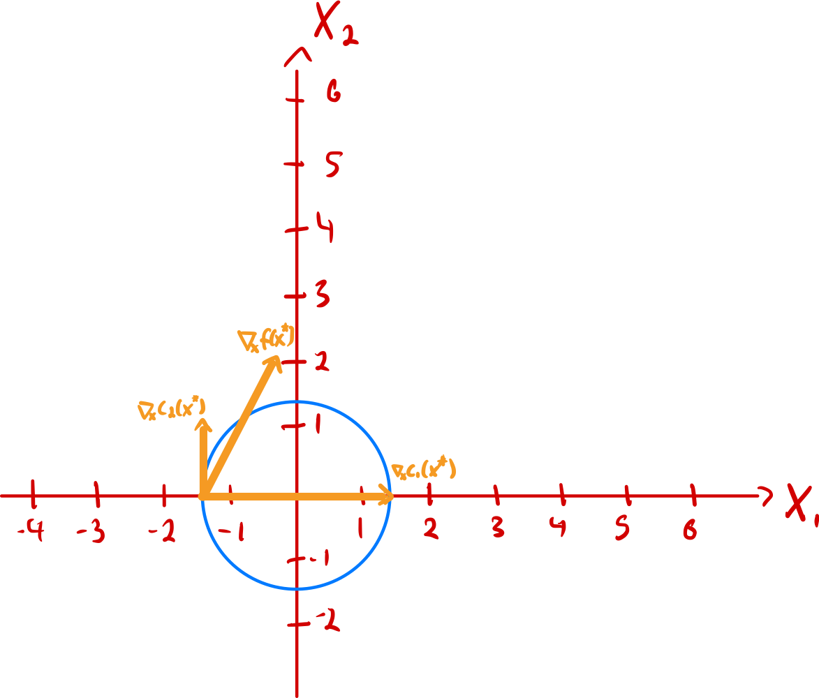
Aka the optimal points are

$$x_a^{\ast }=\left[\begin{array}{cc}\frac{\sqrt{2}}{2}& \frac{\sqrt{2}}{2}\end{array}\right]\cap x_b^{\ast }=\left[\begin{array}{cc}-\frac{\sqrt{2}}{2}& -\frac{\sqrt{2}}{2}\end{array}\right]$$

Illustrating the gradients gives us the following plots for $x_b$ and $x_a$ respectively.

---