Matlab Assignment 4

Training Neural Networks using Steepest Descent

Task

Implement a steepest descent algorithm to train the neural network

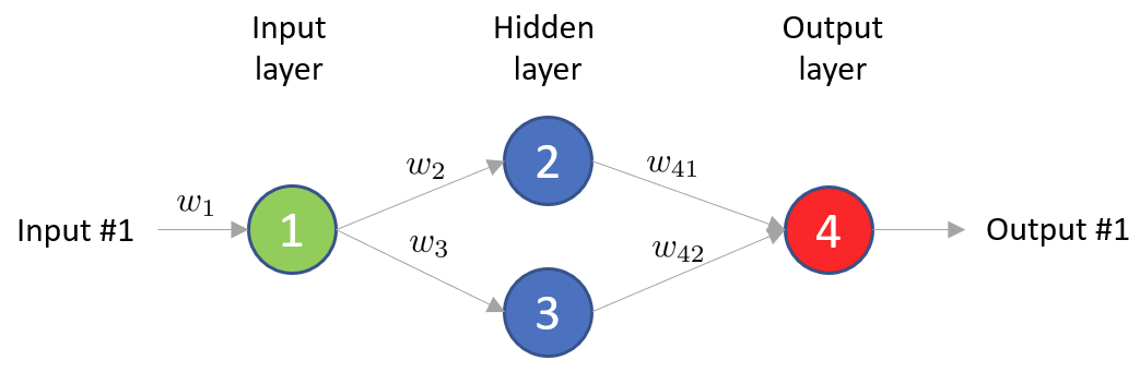
Given this fully connected neural network We want to train it, aka solve the following minimization problem

$$\underset{\theta }{\min }E(\theta )=\sum _{i=1}^N\frac{1}{2}(y_i-f_{NN}(x_i;\theta ){)}^2$$

Note that this is an Unconstrained Optimization problem, but since this network is very small we can use standard gradients algorithms without “cheating.”

Important stuff to notice

$f_{NN}$ is the neural network, and ${\nabla }_{\theta }{f}_{NN}(x_i;\theta )$ is the gradient of the neural network with respect to the parameters.

Solution

By doing the following changes in the main for loop

% Data
x = 0:0.2:2*pi;
rng('default');
y = .1*(x + cos(x) + 1) + .1*rand(size(x));
 
N = size(x,2); % Number of data points
 
n_theta = 9; % Number of parameters
 
% NN parameters
alpha = .1;
n_iter = 2000;
 
% Allocate storage
ES = zeros(1,n_iter+1);
theta = zeros(n_theta,n_iter+1);
 
theta(:,1) = rand(n_theta,1); % initial value of parameter
 
% Initial value of E
E = 0;
for i = 1:N,
    E = E + .5* (y(i) - f_NN(x(i),theta) ).^2;
end
ES(1) = E; % ES stores the value of the objective function for each iteration, E for plotting
 
% Steepest descent algorithm
for k=1:n_iter,
    % Initialize gradient accumulator
    dE_dtheta = zeros(n_theta,1);
    
    % Sum over all data points to calculate gradient
    for i = 1:N,
        % Compute gradient of the neural network output with respect to parameters
        [dydtheta_i, y_i] = gradient_f_NN(x(i),theta(:,k));
        % Compute the error derivative for this data point
        e_i = y(i) - y_i;
        % Accumulate the gradient of the error function
        dE_dtheta = dE_dtheta + (-e_i * dydtheta_i);
    end
    
    % Update parameters using steepest descent
    theta(:,k+1) = theta(:,k) - alpha * dE_dtheta;
    
    % Recalculate value of E for the updated parameters
    E = 0;
    for i = 1:N,
        E = E + .5* (y(i) - f_NN(x(i),theta(:,k+1)) )^2;
    end
    ES(k+1) = E;
end
 
theta_opt = theta(:,end);
 
figure(1)
plot(0:n_iter,ES);
xlabel('Iteration'); ylabel('E');
 
figure(2);
plot(x,y); hold on;
plot(x,f_NN(x,theta_opt),'m--'); hold off
xlabel('x'); ylabel('y');
 
function y = f_NN(x,theta)
% Do a forward pass of a 1-2-1 Neural Network.
% 
%   x           input
%   theta       parameters theta = (w1, b1, w2, b2, w3, b3, w41, w42, b4)
%   
%   y           output
 
% Activation function ("logistic")
sigma = @(r) 1./(1+exp(-r));
 
w1 = theta(1);
b1 = theta(2);
w2 = theta(3);
b2 = theta(4);
w3 = theta(5);
b3 = theta(6);
w41 = theta(7);
w42 = theta(8);
b4 = theta(9);
 
y1 = sigma(w1*x + b1);
y2 = sigma(w2*y1 + b2);
y3 = sigma(w3*y1 + b3);
y = sigma(w41*y2 + w42*y3 + b4);
end
 
function [dydtheta, y] = gradient_f_NN(x,theta)
% Calculate the gradient of the 1-2-1 NN wrt parameters.
% Note: This is an inefficient implementation, using "forward" (chain rule)
% differentiation. "Reverse" differentiation aka back propagation 
% would be more efficient, but the difference is not
% significant for this small example. Machine learning frameworks use 
% reverse mode of automatic differentiation to compute these derivatives.
% 
%   x           input
%   theta       parameters theta = (w1, b1, w2, b2, w3, b3, w41, w42, b4)
%   
%   y           output
%   dydtheta    gradient of y wrt theta
 
% Activation function ("logistic")
sigma = @(r) 1./(1+exp(-r));
 
% Derivative of activation function (as a function of the output of the sigma function)
dsigmadr = @(sigma) sigma*(1-sigma);
 
w1 = theta(1);
b1 = theta(2);
w2 = theta(3);
b2 = theta(4);
w3 = theta(5);
b3 = theta(6);
w41 = theta(7);
w42 = theta(8);
b4 = theta(9);
 
y1 = sigma(w1*x + b1);
y2 = sigma(w2*y1 + b2);
y3 = sigma(w3*y1 + b3);
y = sigma(w41*y2 + w42*y3 + b4);
 
dydtheta = [
    dsigmadr(y)*w41*dsigmadr(y2)*w2*dsigmadr(y1)*x + dsigmadr(y)*w42*dsigmadr(y3)*w3*dsigmadr(y1)*x; % dydw1
    dsigmadr(y)*w41*dsigmadr(y2)*w2*dsigmadr(y1) + dsigmadr(y)*w42*dsigmadr(y3)*w3*dsigmadr(y1); % dydb1
    dsigmadr(y)*w41*dsigmadr(y2)*y1; % dydw2
    dsigmadr(y)*w41*dsigmadr(y2); % dydb2
    dsigmadr(y)*w42*dsigmadr(y3)*y1; % dydw3
    dsigmadr(y)*w42*dsigmadr(y3); % dydb3
    dsigmadr(y)*y2; % dydw41
    dsigmadr(y)*y3; % dydw42
    dsigmadr(y); % dydb4
    ];
   
end
 
 
 

NOTE:

dE_dtheta - $\frac{\partial }{\partial \theta }E$ / ${\nabla }_{\theta }E$

• Represents the gradient of the error function $E$ with respect to the parameters $\theta$

dydtheta - $\frac{\partial }{\partial \theta }y$ / ${\nabla }_{\theta }y$

• Represents the gradient of output $y$ with respect to the parameters $\theta$

dydtheta_i - $\frac{\partial }{\partial \theta }{y}_i$ / ${\nabla }_{\theta }{y}_i$

• Represents the gradient of the output in a specific input data point $i$, with respect to the parameters $\theta$.

The core formula in updating the parameters is found in line 43:

Core formula

${\theta }_{new}={\theta }_{old}-\alpha {\nabla }_{\theta }E$

$\downarrow$

theta(:,k+1) = theta(:,k) - alpha * dE_dtheta;

The last iteration is the optimal set of parameters.