Assignment 4

Resources: sf2024.pdf Ch. 6

---

Task 1: Gaussian mixture reduction

Given

Gaussian Mixtures

Resources: page=109 Ch. 6.3

---

A Gaussian mixture is a function on the form

$$f(x)=\sum _{i=1}^M{w}^i\mathcal{N}(x;{\mu }^i{P}^i)$$

Where ${\sum }_{i=1}^M{w}^i=1$ and $w^i\ge 0\forall i$

• $w^i$ is used for what is called the normalization requirement, and ensures that the mixture integrates to one (making $f(x)$ a valid pdf).

Link to original

(Both a and b should’ve be optimized using numpy if there were runtime requirements)

In a and b, the following helper functions were used

def statecv_to_numpy(state: StateCV) -> np.ndarray:
    """Convert a StateCV object to a numpy array."""
    # Convert position and velocity components to a numpy array
    pos_array = np.array([state.x, state.y])
    vel_array = np.array([state.u, state.v])
    
    # Concatenate position and velocity arrays (or choose the part you need)
    return np.concatenate((pos_array, vel_array))

def measpos_to_numpy(meas: MeasPos) -> np.ndarray:
    """Convert a MeasPos object to a numpy array."""
    return np.array([meas.x, meas.y])

a)

The mean of a Gaussian mixture is given by Eq 6.24

$$\bar{\mu }=\sum _{i=1}^M{w}^i{\mu }^i$$

Where $w^i$ are the weights corresponding to the means ${\mu }^i$ in the mixture.

def mean(self):
        """Find the mean of the gaussian mixture."""
        mean = 0
        for i in range(len(self.gaussians)):
            mu_i = self.gaussians[i].mean
            
            # Convert StateCV and MeasPos objects to numpy arrays
            if isinstance(mu_i, StateCV):
                mu_i = statecv_to_numpy(mu_i)
            elif isinstance(mu_i, MeasPos):
                mu_i = measpos_to_numpy(mu_i)
 
            w_i = self.weights[i]
            mean += w_i * mu_i
 
        return mean

b)

The covariance of a Gaussian mixture is given by Eq. 6.25

$$\bar{P}=\sum _{i=1}^M{w}^i{P}^i+\tilde{P}$$

Where $w^i$ are the weights corresponding to the covariances $P^i$ in the mixture, and $\tilde{P}$ is the spread-of-the-innovations terms which is given by

$$\tilde{P}=\sum _{i=1}^M{w}^i({\mu }^i-\bar{\mu })({\mu }^i-\bar{\mu }{)}^T=\sum _{i=1}^M{w}^i{\mu }^i({\mu }^i{)}^T-\bar{\mu }{\bar{\mu }}^T$$

def cov(self):
        """Find the covariance of the gaussian mixture.
        Hint: Use (6.25) from the book."""
 
        mu_bar = self.mean()
        cov = 0
        P_tilde = 0 
 
        for i in range(len(self.gaussians)):
            mu_i = self.gaussians[i].mean
            if isinstance(mu_i, StateCV):
                mu_i = statecv_to_numpy(mu_i)
 
            w_i = self.weights[i]
            P_i = self.gaussians[i].cov
            
            cov += w_i * P_i
 
            P_tilde += w_i * (mu_i - mu_bar) @ (mu_i - mu_bar).T
 
        cov += P_tilde 
        return cov

c)

i. $w=\left\{\frac{1}{3},\frac{1}{3},\frac{1}{3}\right\},\mu =\{0,2,4.5\},P=\{1^2,1^2,1^2\}$

Since all the Gaussians have identical weights and covariances, we would like to combine the Gaussians that have the closest means, which in this case is Gaussian 0 and 1. 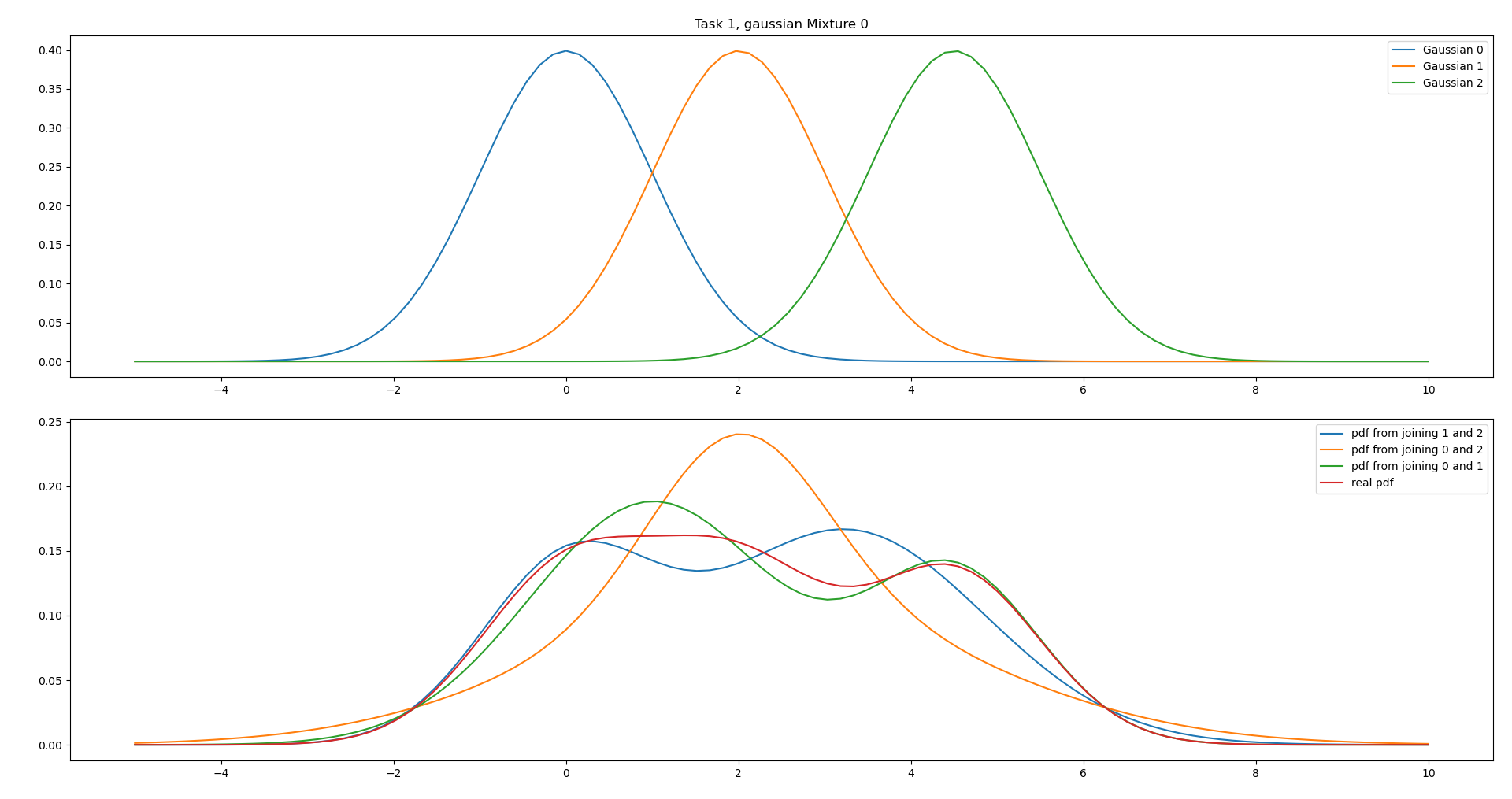From the plot we can see that this matches the real pdf the best.

$$\begin{array}{rl}{w}_{0,1}& =w_0+w_1=\frac{2}{3}\\ {\mu }_{0,1}& =\frac{w_0}{w_{0.1}}{\mu }_0+\frac{w_1}{w_{0.1}}{\mu }_1=1\\ {\sigma }_{0,1}^2& =\frac{w_0}{w_{0.1}}{\sigma }_0^2+\frac{w_1}{w_{0.1}}{\sigma }_1^2+\frac{w_1{w}_2}{(w_1+w_2{)}^2}({\mu }_1-{\mu }_2{)}^2={\sqrt{2}}^2\end{array}$$

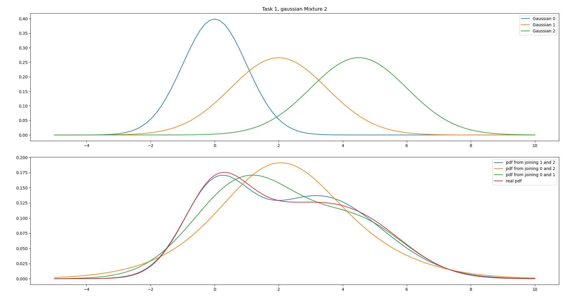
ii. $w=\left\{\frac{1}{6},\frac{4}{6},\frac{1}{6}\right\},\mu =\{0,2,4.5\},P=\{1^2,1^2,1^2\}$

We can see from the parameters that the weights of Gaussian 0 and 2 are very small, and it might therefore be a good decision to combine these (even though the means are far apart) 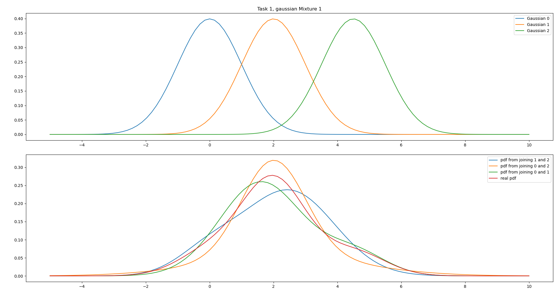We can see from the plot that this represents the real pdf fairly well and has the same expected value.

$$\begin{array}{rl}{w}_{0,2}& =\frac{1}{6}+\frac{1}{6}=\frac{1}{3}\\ {\mu }_{0,2}& =\cdots =\frac{9}{4}\\ {\sigma }_{0,2}^2& =\cdots \approx 2.46\end{array}$$

iii. $w=\left\{\frac{1}{3},\frac{1}{3},\frac{1}{3}\right\},\mu =\{0,2,4.5\},P=\{1^2,1.5^2,1.5^2\}$

This case is very similar to i., however with different covariances. If we combine Gaussian 0 and 1 it will become “to stretched” to the left. We can see from the plot that combining Gaussian 1 and 2 is therefore the most accurate combiniation due to the high covariances.

$$\begin{array}{rl}{w}_{1,2}& =\frac{2}{3}\\ {\mu }_{1,2}& =\frac{13}{4}\\ {\sigma }_{1,2}^2& \approx 1.95\end{array}$$

iv. $w=\left\{\frac{1}{3},\frac{1}{3},\frac{1}{3}\right\},\mu =\{0,0,2.5\},P=\{1^2,1.5^2,1.5^2\}$

Similar case as in iii., however the mean of Gaussian 0 and 1 are the same. However it is not obvious from the parameters alone which is the best. 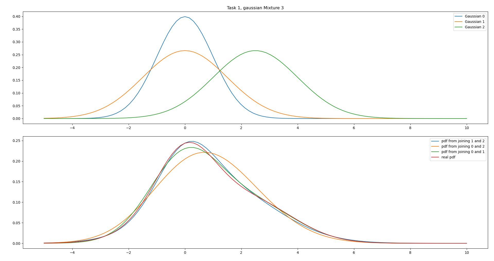We can see that combining both Gaussian 0 and 1, and Gaussian 1 and 2 gives good results, but the peak of 0 and 1 is too low. Therefore combining 1 and 2 is the best option.

$$\begin{array}{rl}{w}_{1,2}& =\frac{2}{3}\\ {\mu }_{1,2}& =1.25\\ {\sigma }_{1,2}^2& =1.95\end{array}$$

Task 2: Measurement likelihood of the interacting multiple model filter and particle filter

Resources:

• page=106 Ch 6.2
• The Hybrid State Concept

a)

b)

Task 3: Implement an IMM class

a)

Which we solve using the following code

def calculate_mixings(self, x_est_prev: GaussianMixture[StateCV],
                          dt: float) -> np.ndarray:
        """Calculate the mixing probabilities, following step 1 in (6.4.1).
 
        The output should be on the following from:
        $mixing_probs[s_{k-1}, s_k] = \mu_{s_{k-1}|s_k}$
        """
        pi_mat = self.dynamic_model.get_pi_mat_d(dt)  # the pi in (6.6)
        prev_weights = x_est_prev.weights  # \mathbf{p}_{k-1}
 
        mixing_probs = pi_mat * prev_weights.reshape(-1, 1)
 
        # Each columnd represents different s_k, normalize the columns.
        mixing_probs /= np.sum(mixing_probs, axis=0)
 
        return mixing_probs

b)

def mixing(self,
               x_est_prev: GaussianMixture[StateCV],
               mixing_probs: GaussianMixture[StateCV]
               ) -> Sequence[MultiVarGauss[StateCV]]:
        """Calculate the moment-based approximations, 
        following step 2 in (6.4.1). 
        Should return a gaussian with mean=(6.34) and cov=(6.35).
 
        Hint: Create a GaussianMixture for each mode density (6.33), 
        and use .reduce() to calculate (6.34) and (6.35).
        """
        moment_based_preds = []
        for i in range(len(x_est_prev)):
            mixture = GaussianMixture[StateCV](
                weights = mixing_probs[:, i], 
                gaussians=x_est_prev.gaussians
            )
            momend_based_pred = mixture.reduce()
            moment_based_preds.append(momend_based_pred)
 
        return moment_based_preds 

c)

def mode_match_filter(self,
                          moment_based_preds: GaussianMixture[StateCV],
                          z: MeasPos,
                          dt: float
                          ) -> Sequence[OutputEKF]:
        """Calculate the mode-match filter outputs (6.36),
        following step 3 in (6.4.1). 
 
        Hint: Use the EKF class from the top of this file.
        The last part (6.37) is not part of this
        method and is done later."""
        ekf_outs = []
 
        for i, x_prev in enumerate(moment_based_preds):
            out_ekf = EKF(self.dynamic_model[i], self.sensor_model).step(x_prev, z, dt)
            ekf_outs.append(out_ekf)
 
        return ekf_outs

d)

def update_probabilities(self,
                             ekf_outs: Sequence[OutputEKF],
                             z: MeasPos,
                             dt: float,
                             weights: np.ndarray
                             ) -> np.ndarray:
        """Update the mixing probabilities,
        using (6.37) from step 3 and (6.38) from step 4 in (6.4.1).
 
        Hint: Use (6.6)
        """
        pi_mat = self.dynamic_model.get_pi_mat_d(dt)
 
        weights_pred = pi_mat.T @ weights.reshape(-1,1)  # use (6.6)
        z_probs = np.array([ekf_outs[i].z_est_pred.pdf(z) for i in range(len(ekf_outs))])
 
        weights_upd = (z_probs * weights_pred) / np.sum(z_probs * weights_pred)
 
        return weights_upd

e)

Combining the previous tasks gives us the following function

def step(self,
             x_est_prev: GaussianMixture[StateCV],
             z: MeasPos,
             dt) -> GaussianMixture[StateCV]:
        """Perform one step of the IMM filter."""
        mixing_probs = self.calculate_mixings(x_est_prev, dt)
        momend_based_preds = self.mixing(x_est_prev, mixing_probs)
        ekf_outs = self.mode_match_filter(momend_based_preds, z, dt)
        weights_upd = self.update_probabilities(ekf_outs, z, dt, x_est_prev.weights)
 
        x_est_upd = GaussianMixture(weights_upd, 
                                        [out.x_est_upd for out in ekf_outs])
        
        x_est_pred = GaussianMixture(x_est_prev.weights,
                                        [out.x_est_pred for out in ekf_outs])
 
        z_est_pred = GaussianMixture(x_est_prev.weights,
                                        [out.z_est_pred for out in ekf_outs])
 
        return x_est_upd, x_est_pred, z_est_pred

Task 4: Tune an IMM

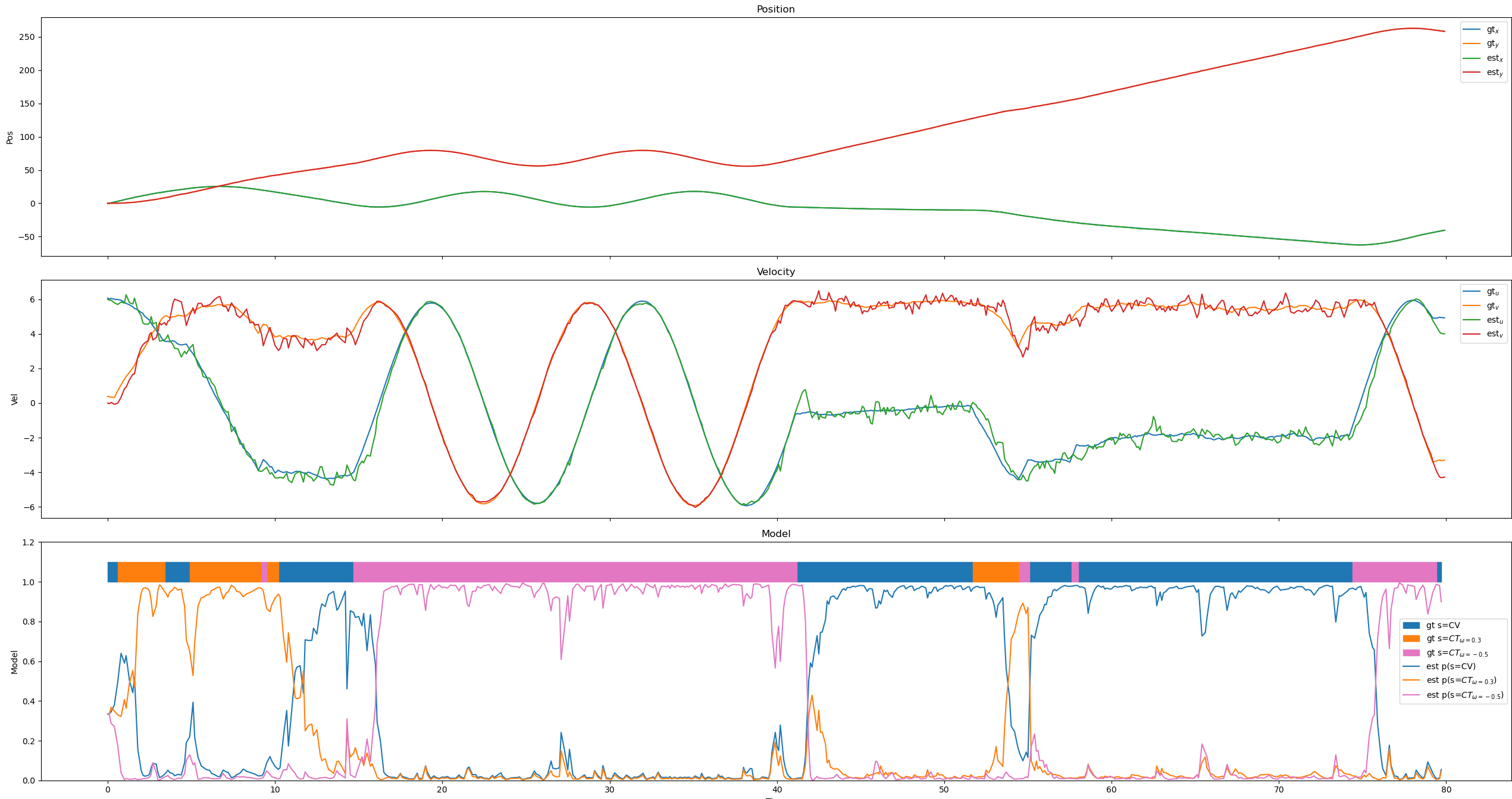
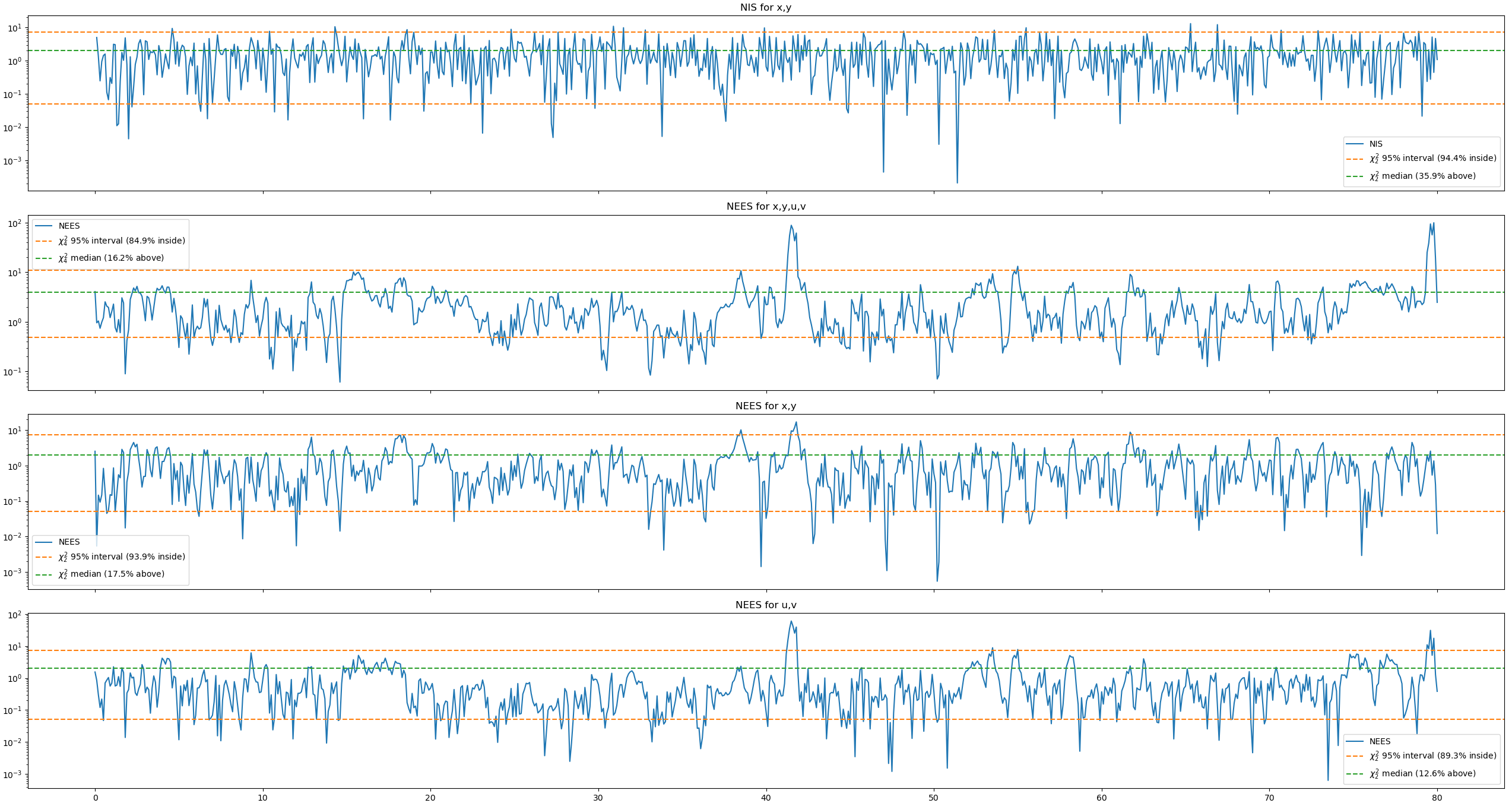
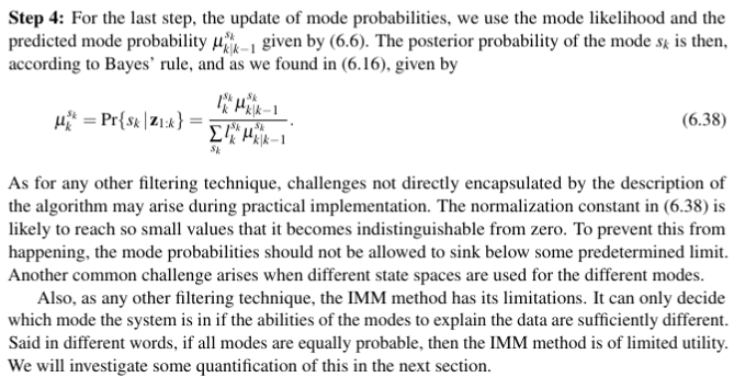
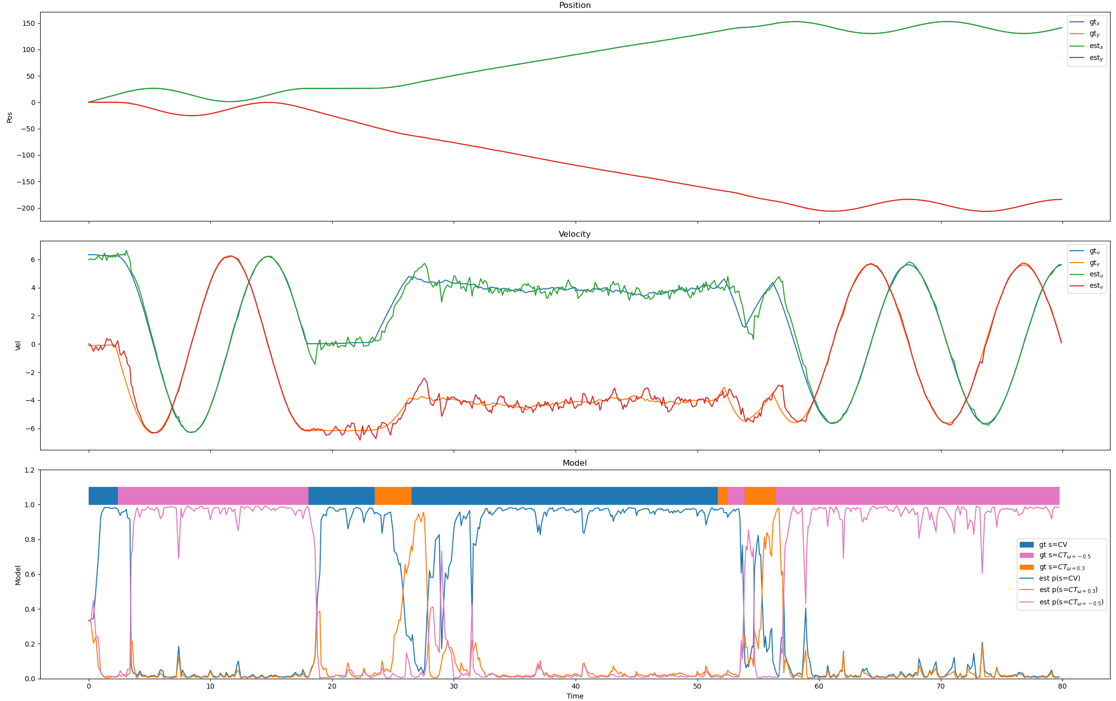
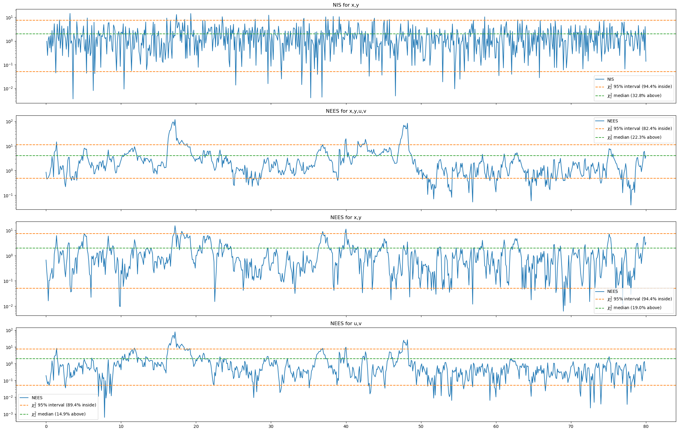
a)

This is the response before changing the parameters.

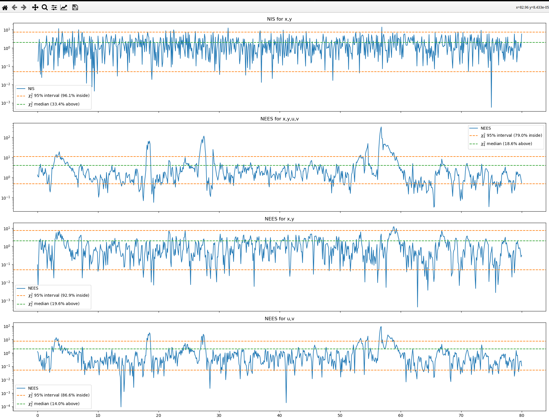
Changing the standard deviation in the position sensor gives

Changing the std in the CV and first CT model gives

b)