Assignment 3

Resources:

• page=53 Ch. 4

---

Task 1: Bayesian Estimation of an Existence Variable

a)

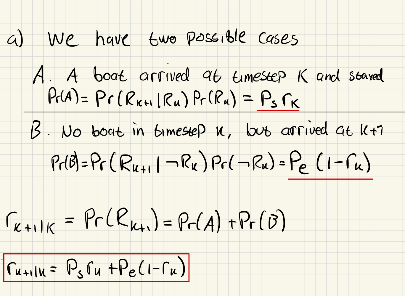
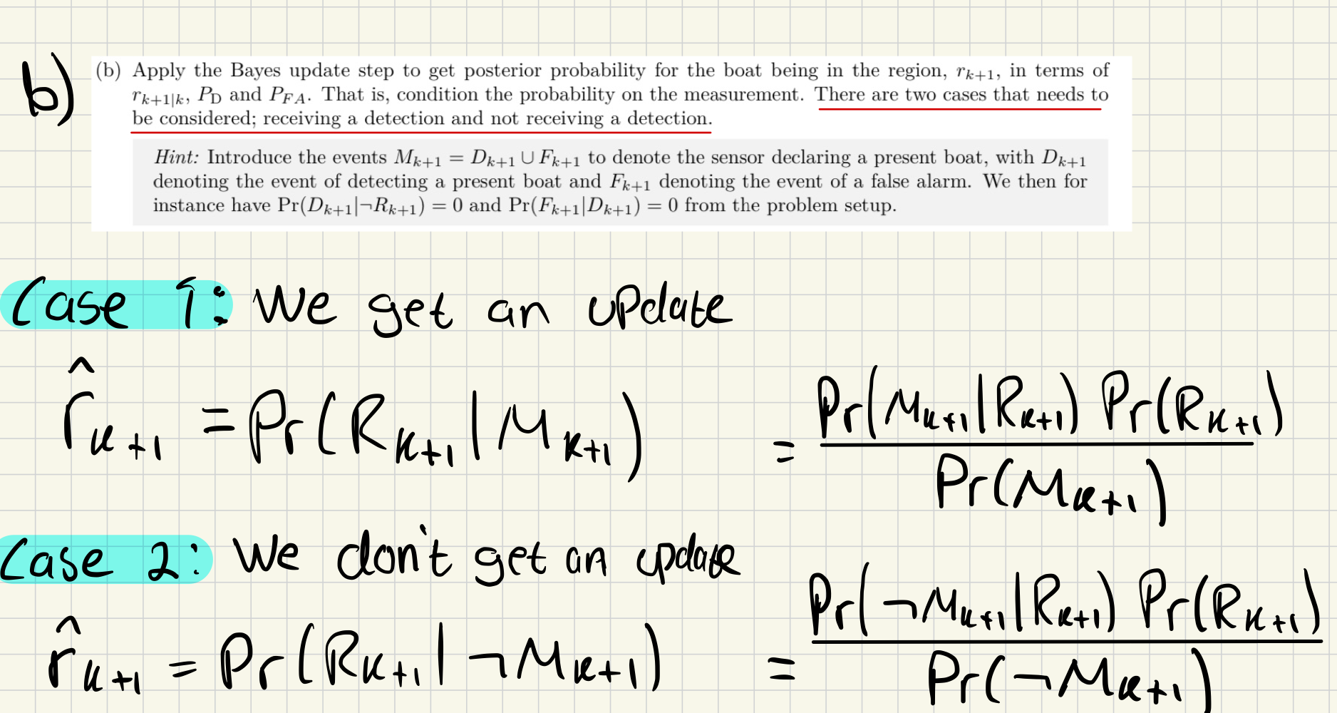
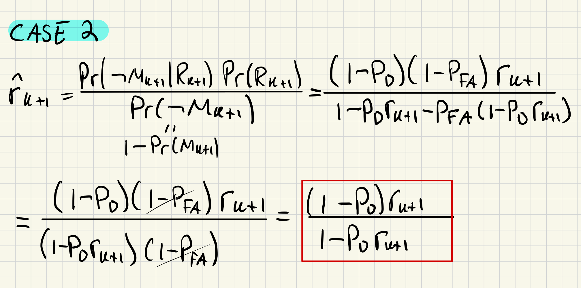
b)

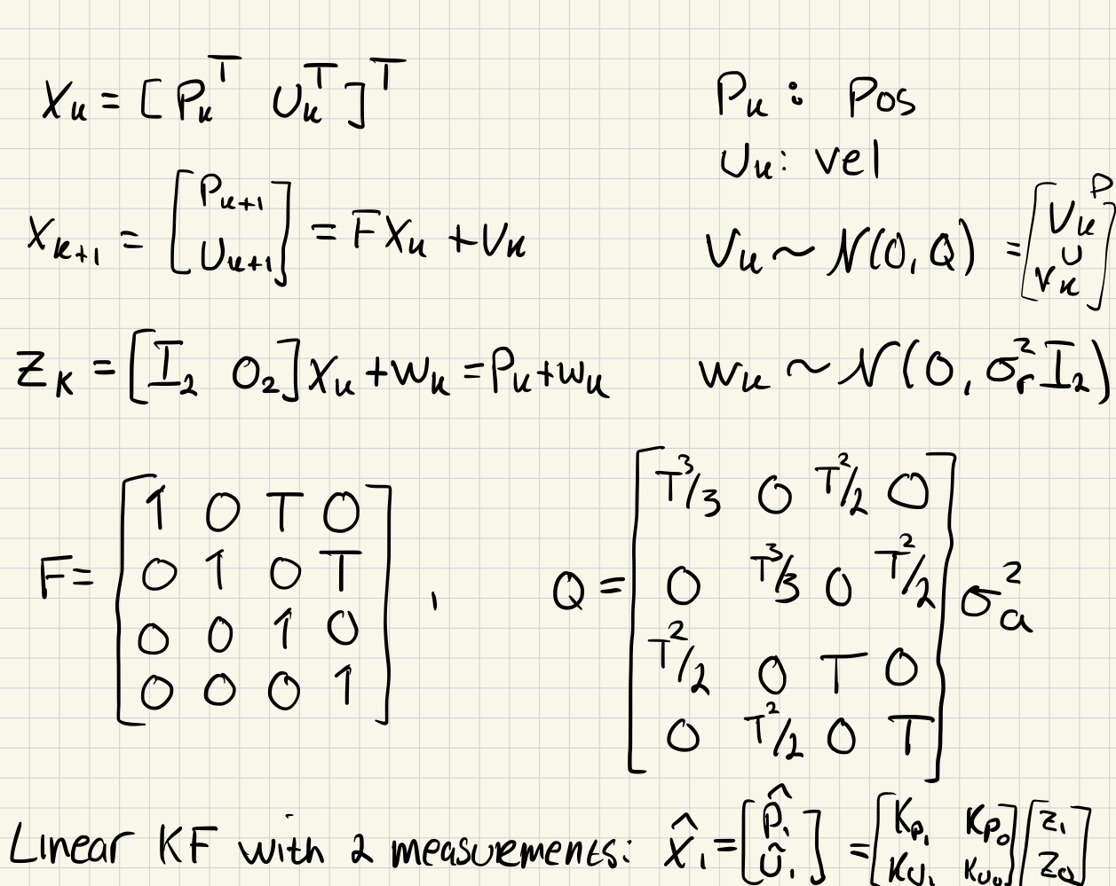
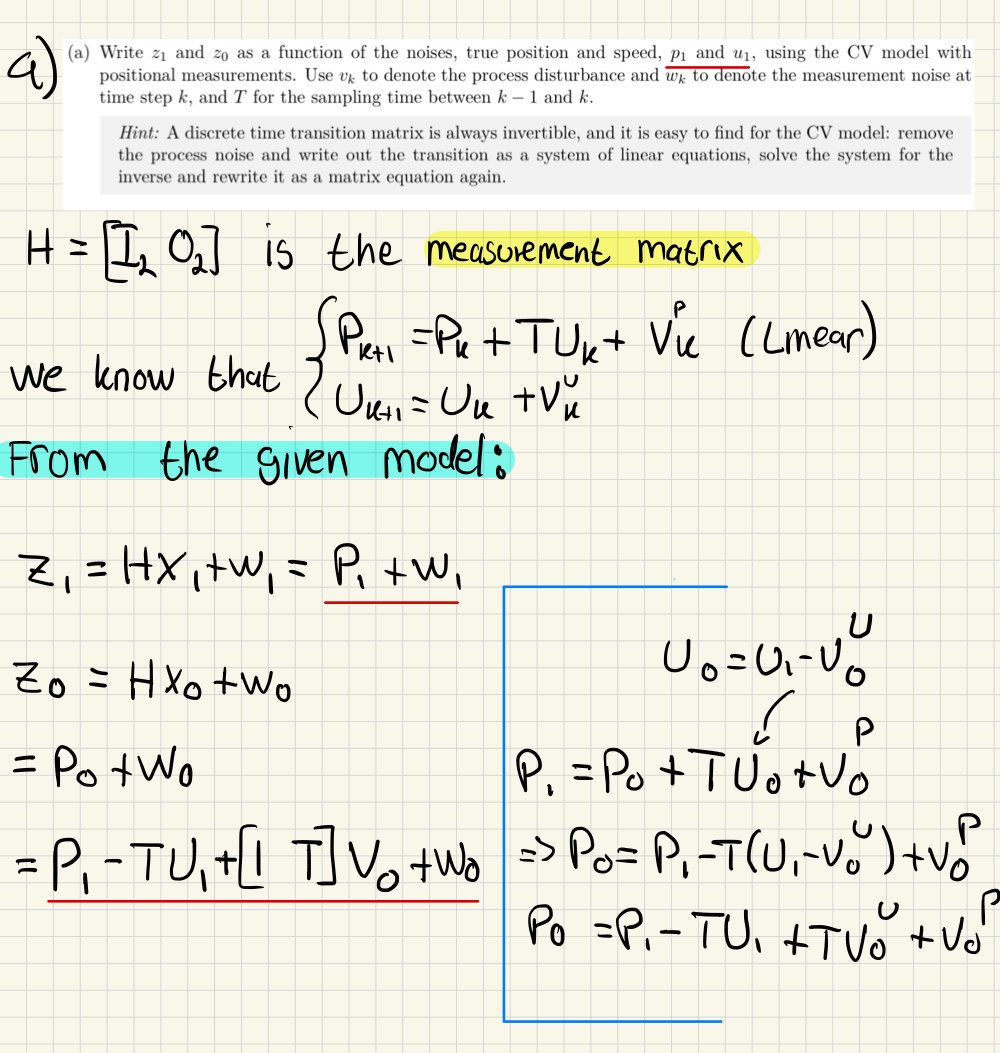
Task 2: KF Initialization of CV Model Without a Prior

KF - Kalman Filter CV model - Assuming nearly constant velocity

$F$ and $Q$ defined in Eq. 4.64 (page=67)

---

a)

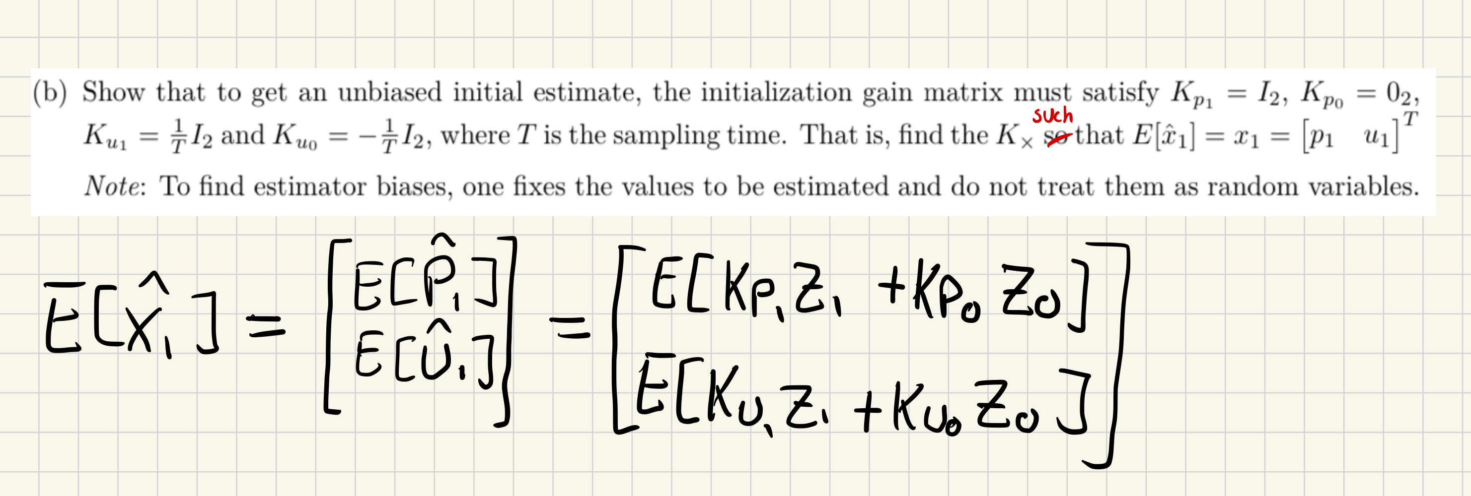
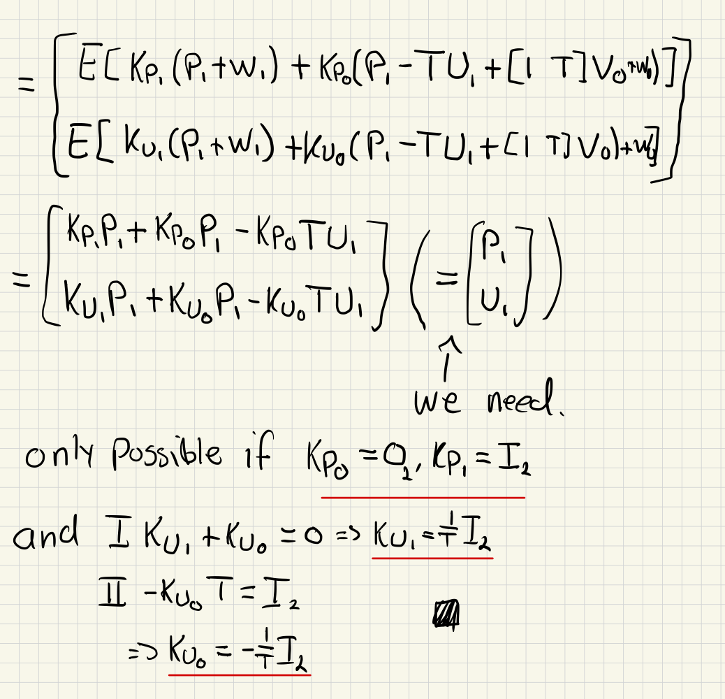
b)

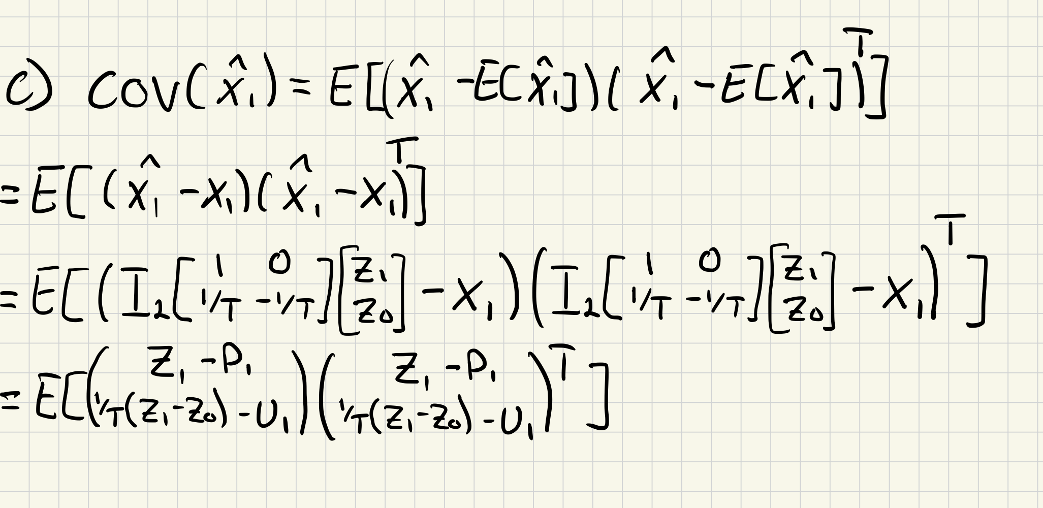
c)

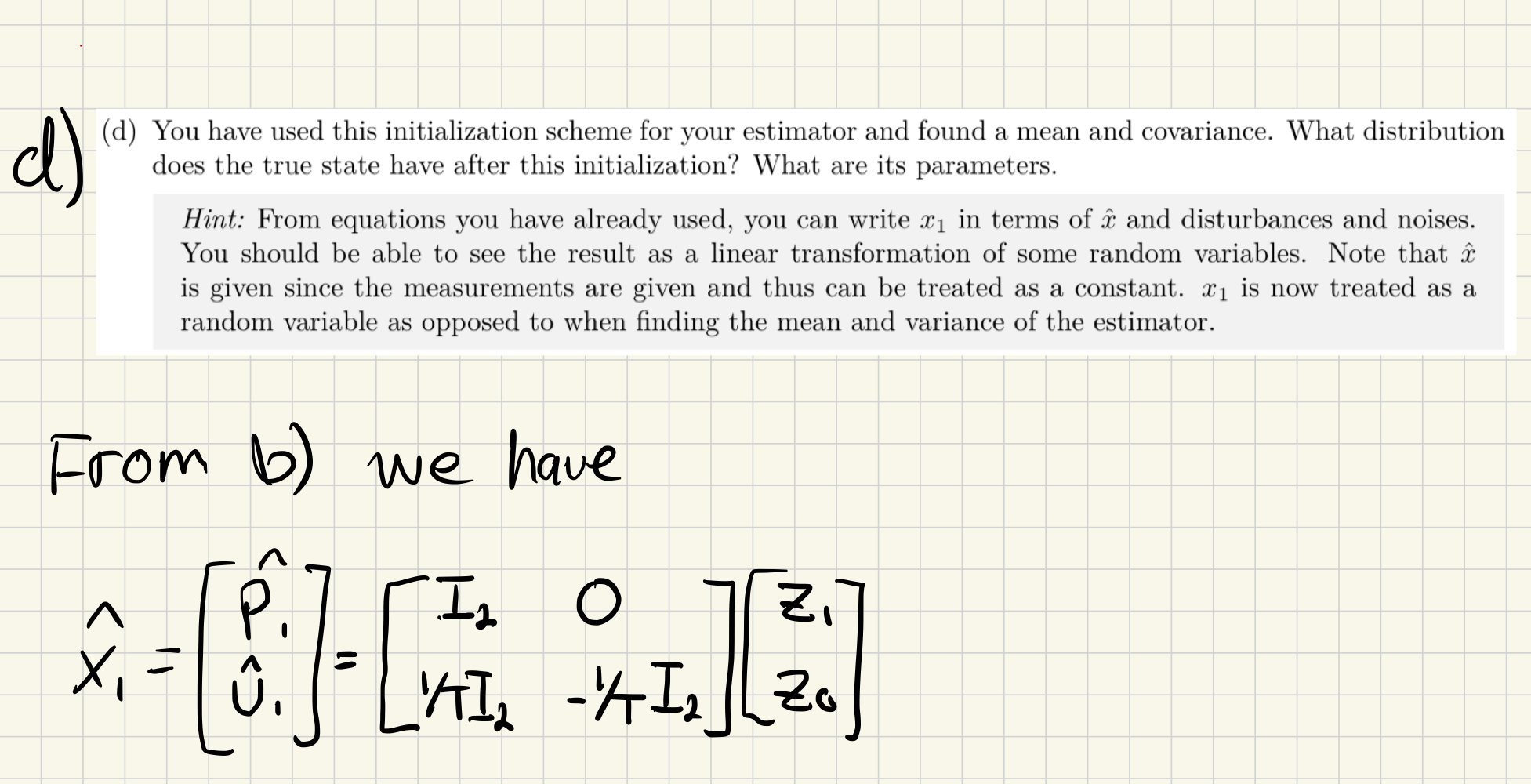
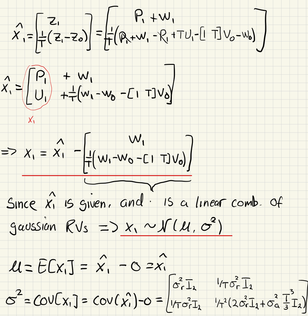
d)

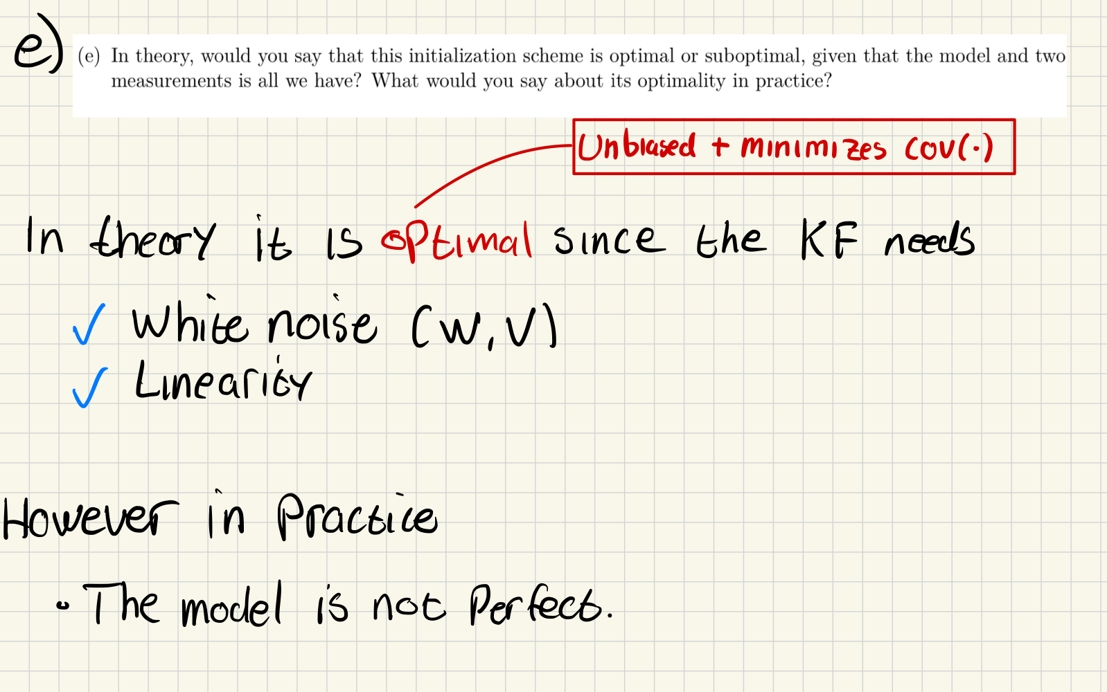
e)

f)

Using the results from task 2c, we can finish implementing initialize.get_init_CV_state.

def get_init_CV_state(meas0: Measurement2d, meas1: Measurement2d,
                      ekf_params: EKFParams) -> MultiVarGauss:
    """This function will estimate the initial state and covariance from
    the two first measurements"""
    dt = meas1.dt
    z0, z1 = meas0.value, meas1.value
    sigma_a = ekf_params.sigma_a
    sigma_z = ekf_params.sigma_z
 
    K_p = np.hstack((np.identity(2), np.zeros((2,2))))
    K_u = np.hstack(((1/dt)*np.identity(2), -(1/dt)*np.identity(2)))
 
    K_x = np.vstack((K_p, K_u))
    z = np.hstack((np.array(z1), np.array(z0)))
    R = (sigma_z**2) * np.identity(2)
 
    mean = K_x @ z  # x_hat_1
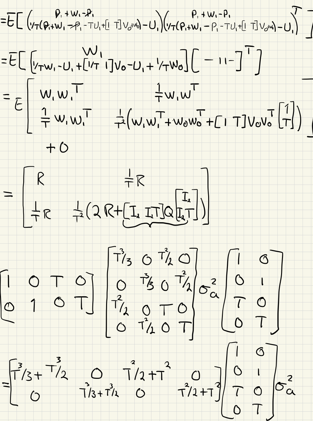
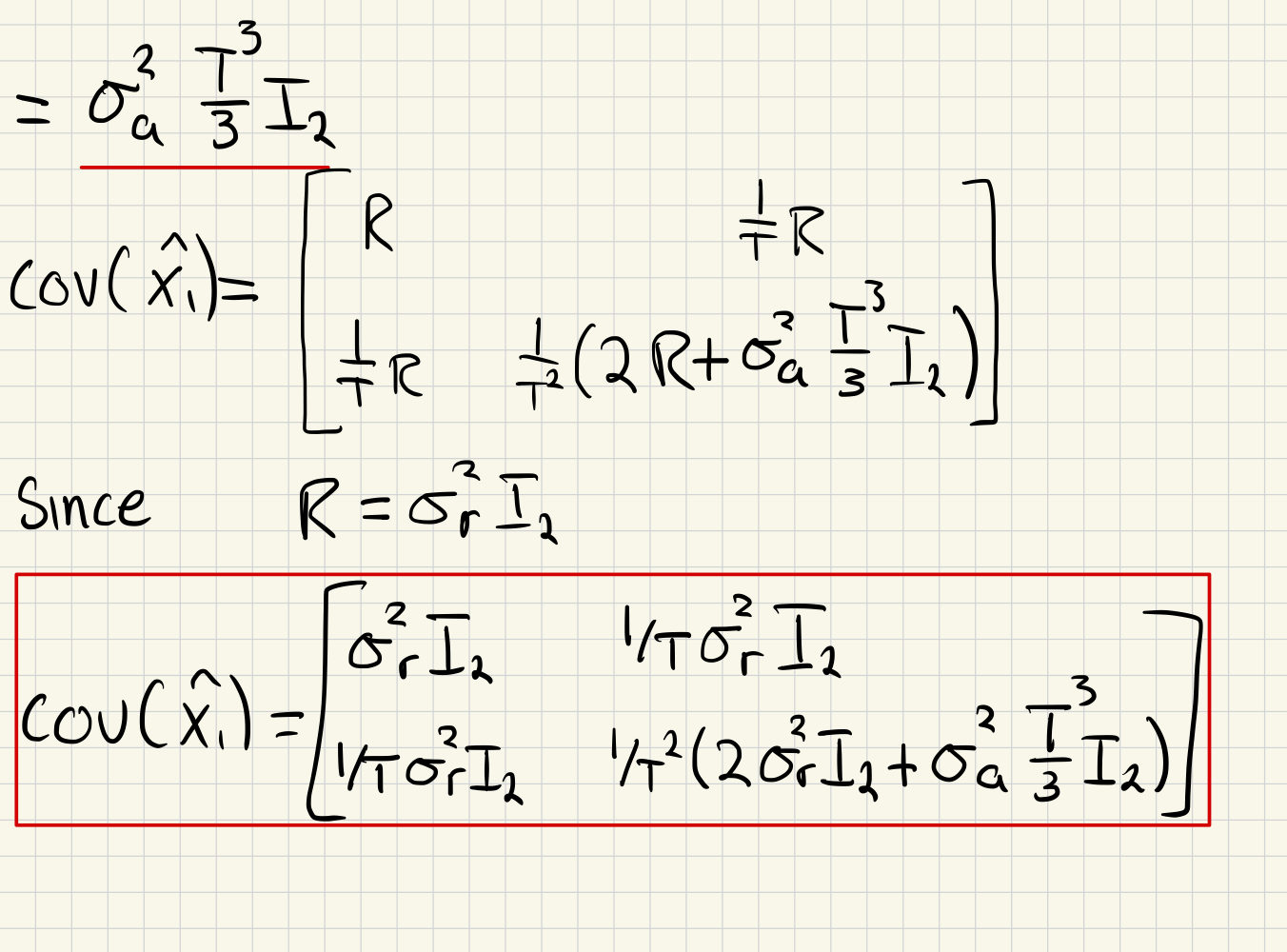
    cov = np.block([ # Covariance matrix from 2c
        [R, (1/dt) * R], 
        [(1/dt) * R, (1/dt)**2 * (2 * R + (sigma_a**2) * (dt**3) / 3 * np.identity(2))] 
    ]) 
 
    init_state = MultiVarGauss(mean, cov)
 
    return init_state

Task 3: Make CV dynamic model and position measurement model

a)

def f(self, x: ndarray, dt: float,) -> ndarray:
        """Calculate the zero noise transition from x given dt."""
 
        x_next = self.F(x, dt) @ x # + v (which is zero)
        return x_next

b)

def F(self, x: ndarray, dt: float,) -> ndarray:
        """Calculate the discrete transition matrix given dt
        See (4.64) in the book."""
 
        F = np.eye(4) + dt * np.array([[0,0, 1, 0],[0, 0, 0, 1],[0, 0, 0, 0],[0, 0, 0, 0]])
        return F

c)

def Q(self, x: ndarray, dt: float,) -> ndarray:
        """Calculate the discrete transition Covariance.
        See(4.64) in the book."""
 
        Q = np.array([[dt**3/3, 0, dt**2/2, 0],[0, dt**3/3, 0, dt**2/2],[dt**2/2, 0, dt, 0],[0, dt**2/2, 0, dt]]) * self.sigma_a**2
        return Q

d)

def predict_state(self,
                      state_est: MultiVarGauss,
                      dt: float,
                      ) -> MultiVarGauss:
        """Given the current state estimate, 
        calculate the predicted state estimate.
        See 2. and 3. of Algorithm 1 in the book."""
        x_upd_prev, P = state_est
 
        F = self.F(x_upd_prev, dt)
        Q = self.Q(x_upd_prev, dt)
 
        x_pred = F @ x_upd_prev
        P_pred = F @ P @ F.T + Q
 
        state_pred_gauss = MultiVarGauss(x_pred, P_pred)
 
        return state_pred_gauss

e)

 def h(self, x: ndarray) -> ndarray:
        """Calculate the noise free measurement value of x."""
 
        x_h = self.H(x) @ x
        return x_h

f)

def H(self, x: ndarray) -> ndarray:
"""Get the measurement matrix at x."""
 
H = np.hstack((np.identity(2), np.zeros((2,2))))
 
return H

g)

def R(self, x: ndarray) -> ndarray:
        """Get the measurement covariance matrix at x."""
 
        R = self.sigma_z**2 * np.identity(2)
        return R

h)

def predict_measurement(self,
                            state_est: MultiVarGauss
                            ) -> MultiVarGauss:
        """Get the predicted measurement distribution given a state estimate.
        See 4. and 6. of Algorithm 1 in the book.
        """
        x_hat, P = state_est
 
        z_hat = self.H(x_hat) @ x_hat
        H = self.H(x_hat)
        S = H @ P @ H.T + self.R(x_hat)  
 
        measure_pred_gauss = MultiVarGauss(z_hat, S)
 
        return measure_pred_gauss

Task 4: Implement EKF in Python

@dataclass
class ExtendedKalmanFilter:
    dyn_modl: WhitenoiseAcceleration2D
    sens_modl: CartesianPosition2D
 
    def step(self,
             state_old: MultiVarGauss,
             meas: Measurement2d,
             ) -> MultiVarGauss:
        """Given previous state estimate and measurement, 
        return new state estimate.
 
        Relationship between variable names and equations in the book:
        \hat{x}_{k|k_1} = pres_state.mean
        P_{k|k_1} = pres_state.cov
        \hat{z}_{k|k-1} = pred_meas.mean
        \hat{S}_k = pred_meas.cov
        \hat{x}_k = upd_state_est.mean
        P_k = upd_state_est.cov
        """
        state_pred = self.dyn_modl.predict_state(state_old, meas.dt)
        meas_pred = self.sens_modl.predict_measurement(state_pred)
 
        x_hat = state_pred.mean
        P = state_pred.cov
        z_hat = meas_pred.mean
        z = meas.value
        S = meas_pred.cov
 
        H = self.sens_modl.H(x_hat)
        kalman_gain = P @ H.T @ np.linalg.inv(S)
        innovation = z - z_hat
 
        state_upd_mean = x_hat + kalman_gain @ innovation
        state_upd_cov = (np.identity(len(x_hat)) - kalman_gain @ H) @ P
 
        state_upd = MultiVarGauss(state_upd_mean, state_upd_cov)
 
        return state_upd, state_pred, meas_pred

Task 5: Analyse the outputs of the KF

a)

The Normalized Innovations Squared is given by

Link to original

def get_nis(meas_pred: MultiVarGauss, meas: Measurement2d) -> float:
    """Calculate the normalized innovation squared (NIS), this can be seen as 
    the normalized measurement prediction error squared. 
    See (4.66 in the book). 
    Tip: use the mahalanobis_distance method of meas_pred, (3.2) in the book
    """
 
    S = meas_pred.cov
    z = meas.value
    z_hat = meas_pred.mean
 
    innovation = z - z_hat
    nis = innovation.T @ np.linalg.inv(S) @ innovation
 
    return nis

b)

The Normalized Estimation Error Squared is given by

Link to original

def get_nees(state_est: MultiVarGauss, x_gt: np.ndarray):
    """Calculate the normalized estimation error squared (NEES)
    See (4.65 in the book). 
    Tip: use the mahalanobis_distance method of x_gauss, (3.2) in the book
    """
 
    x_hat = state_est.mean
    P = state_est.cov
    NEES = (x_hat - x_gt).T @ np.linalg.inv(P) @ (x_hat - x_gt)
 
    return NEES

d)

[!Definition of Commensurate] Corresponding in size or degree; in proportion. ”salary will be commensurate with age and experience”

1. The state errors should be acceptable as zero mean.

• This ensures that the filter is not biased. If it is biased, it might diverge over time.
• This can be checked by placing the system in a known position and looking for drifts

2. The state errors should have magnitude commensurate with the state covariance yielded by the filter.

• This ensures that the filter is not over/under-confident in its estimates. This can lead to poor performance
• This can be checked using NEES. Under is an example from a previous task
  • 

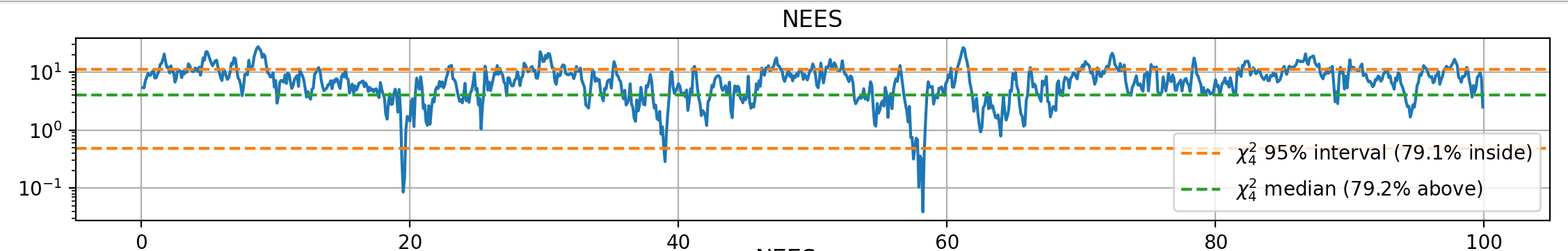
3. The innovations should be acceptable as zero mean.

• The innovation is defined as the difference between the predicted and actual measurement, $\hat{z}-z$. If it is not zero mean, it means that the predictions are biased, and therefore it might not correctly track the states.
• Average of the innovation over many time steps. Should average to zero with sufficiently many samples.

4. The innovations should have magnitude commensurate with the innovation covariance yielded by the filter.

• The innovation covariance reflects uncertainty in the measurements. Same logic as 2
• Can be checked using NIS, and should be checked to neither be too high or too low.

5. The innovations should be acceptable as white

• I don’t understand what is meant by “acceptable as white”