Assignment 2, Part 2

Resources:

• Chapter 7, 10, 15 in Fossen.

---

Objective: In this assignment, you will design a heading autopilot to steer the marine craft model from Assignment 2, Part 1. The autopilot will be tested by adding environmental disturbances in the form of current and wind.

---

Problem 1: Environmental Disturbance

Resources: Chapter 10 in Fossen

a)

We have from equation 10.149 in Fossen that:

$$u_c=V_c\cos ({\beta }_{V_c}-\psi ),v_c=V_c\sin ({\beta }_{V_c}-\psi )$$

Where

• $V_c=\sqrt{u_c^2+v_c^2}=1m/s$, $v$ is the sway velocity
• $r$ is the yaw rate
• $\psi$ is the yaw angle
• ${\beta }_{V_c}$ is the direction of the current
• $(u_c,v_c)$ are the current velocities

Which has been implemented in the Matlab file main.m

b)

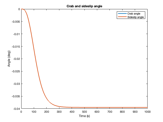
No current

With current

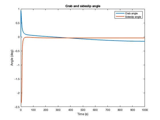
We see in the second plot that when the sideslip angle is zero, the crab angle is non zero. This is because they are directly related, and to stay on the wanted path a crab angle to counteract the current is necessary.

c)

The following changes were done in order to implement the wind moments $Y_{wind}$ and $N_{wind}$ in sway and yaw respectively.

 
% Part 2, 1c) Add wind here 
 
u_w = V_w * cos(beta_w - x(6));
v_w = V_w * sin(beta_w - x(6));
u_rw = x(1) - u_w;
v_rw = x(2) - v_w;
Vrw = sqrt(u_rw^2 + v_rw^2);
gamma_rw = -atan2(v_rw,u_rw);
Ywind = 0.5*rho_a*V_w^2*c_y*sin(gamma_rw)*A_L;
Nwind = 0.5*rho_a*V_w^2*c_n*sin(2*gamma_rw)*A_L*L_oa;
 
if t(i) > 200
	tau_wind = [0 Ywind Nwind]';
else
	tau_wind = [0 0 0]';
end

Where

• $V_w=10$ m/s
• ${\beta }_{V_w}=135^{\circ }$
• ${\rho }_a=1.247kg/m^3$
• $c_y=0.95,c_n=0.15$
• $A_{L_w}=10L_{oa}$, where $L_{oa}$ is the length of the ship

Problem 2: Heading Autopilot

Resources:

• Chapter 7 and 15 in Fossen

a)

From part 1 we know that

$$\begin{array}{rl}{C}_{RB}& =m\left[\begin{array}{ccc}0& -r& -r{x}_g\\ r& 0& -r{y}_g\\ r{x}_g& r{y}_g& 0\end{array}\right]\end{array}$$

and

$$C_A(\nu )=\left[\begin{array}{ccc}0& 0& a_2\\ 0& 0& -a_1\\ -a_2& a_1& 0\end{array}\right]$$

Where $a_1=X_{\dot{u}}u$, and $a_2=Y_{\dot{v}}v+Y_{\dot{r}}r$ (Eq. 6.47 → 6.52).

Linearizing $C_{RB}(\nu )\nu$ and $C_A(\nu )\nu$ around $v=r=0$, and $u=u_d$ we get:

$$C_{RB}^{\ast }\nu =\left[\begin{array}{c}0\\ m{u}_{d}r\\ m{x}_g{u}_{d}r\end{array}\right],C_A^{\ast }\nu =\left[\begin{array}{c}0\\ -X_{\dot{u}}{u}_{d}r\\ u_d(X_{\dot{u}}-Y_{\dot{u}})v-Y_{\dot{r}}{u}_{d}r\end{array}\right]$$

Thus giving us the linearized Coriolis forces as

$$\begin{array}{rl}{C}_{RB}^{\ast }& =\left[\begin{array}{ccc}0& 0& 0\\ 0& 0& m{u}_d\\ 0& 0& m{x}_g{u}_d\end{array}\right]\\ C_A^{\ast }& =\left[\begin{array}{ccc}0& 0& 0\\ 0& 0& -X_{\dot{u}}{u}_d\\ 0& u_d(X_{\dot{u}}-Y_{\dot{u}})& -Y_{\dot{r}}{u}_d\end{array}\right]\end{array}$$

b)

The sway-yaw maneuvering model is given by

$$M{\dot{\nu }}_r+N{\nu }_r=b\delta$$

Where

• $b=b^{\ast }=2u_d[-Y_{\delta },-N_{\delta }{]}^T$
• ${\nu }_r=[v_r,r{]}^T$
• $M\triangleq M_{RB}+M_A$
• $N\triangleq C_{RB}^{\ast }+C_A^{\ast }+D$.

Using the function ss2tf where $A=-M^{-1}N$, $B=M^{-1}b$ and $C^T=[0,1]$ and $d=0$ we get

$$\frac{r}{\delta }(s)=\frac{K(T_{3}s+1)}{(T_{1}s+1)(T_{2}s+1)}(\text{Eq.}7.20)$$

Where $K=0.0075$, $T_1=6.8992$, $T_2=176.7041$, and $T_3=14.0540$.

c)

Using the Nomoto Model we get that the first-order Nomoto model has parameters $T\triangleq T_1+T_2-T_3=169.55$, and $K=0.0075$.

d)

We now want to design a PID controller using pole placement according to Alg 15.1 in Fossen, with the following parameters:

• ${\omega }_b=0.06\text{ rad/s}$
• ${\omega }_{\text{ref}}=0.03\text{ rad/s}$
• $\zeta =1$ - Critical dampening

e)

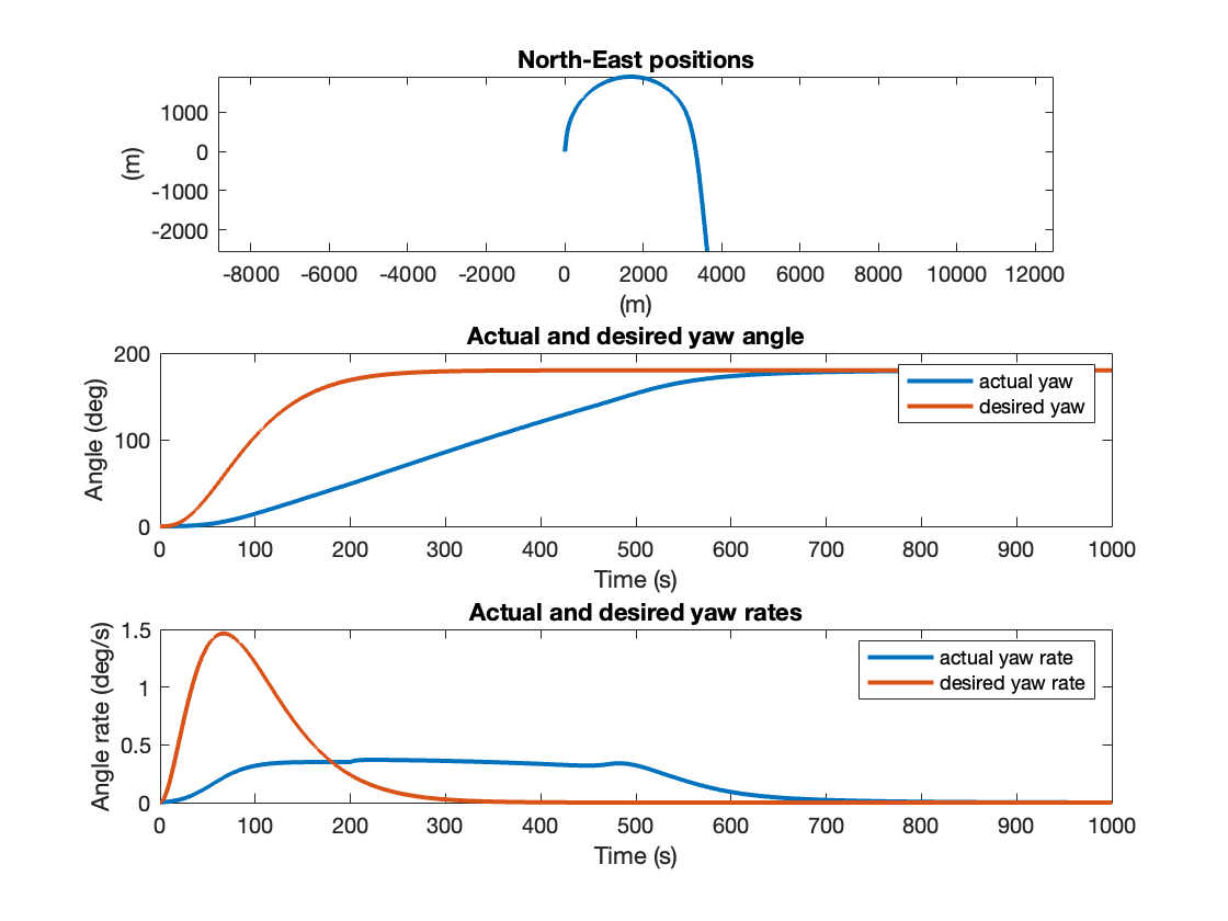
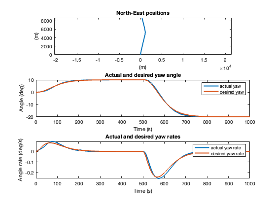
Based on the response we can see signs of integrator wind up in the yaw angle plot where the actual yaw rate keeps increasing even though the desired yaw raw is constant at $200^{\circ }$.

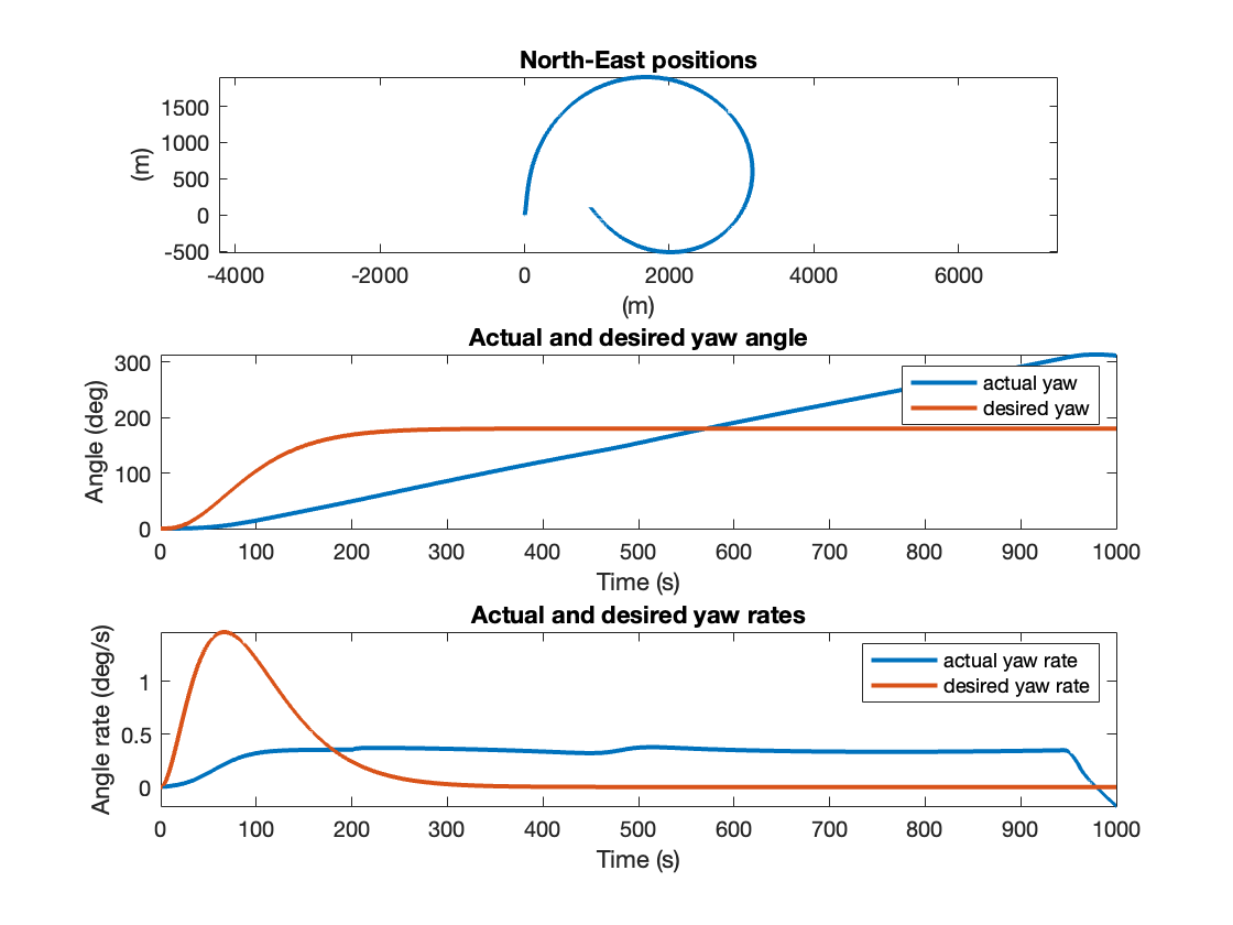
This is due to to saturation in the maximum possible yaw rate which in turn leads to integrator wind up since we integrate the error. This is fixed by turning of the integrator when the system is in saturation. See the Matlab file main.m and the plot.